Chroma Ray Tracer 
Development Blog
Author:Alper Şahıstan(github)
![]()
Introduction
This repository is meant to contain a simple implementation of the ray tracing algorithm. Hopefully will surpass its humble conception. This page will also be used as a blog to update on the development process. Developed for CENG795 course at METU(2019-2020 Spring Semester).
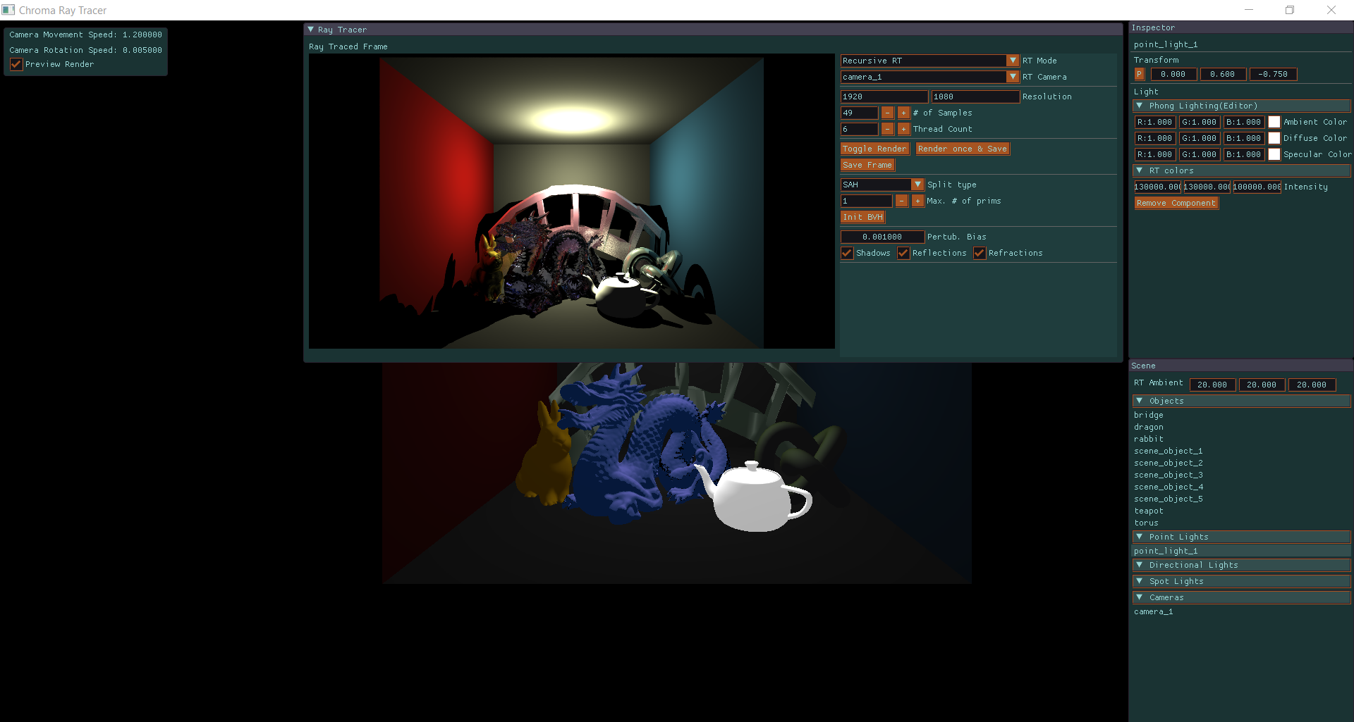
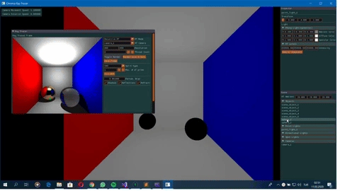
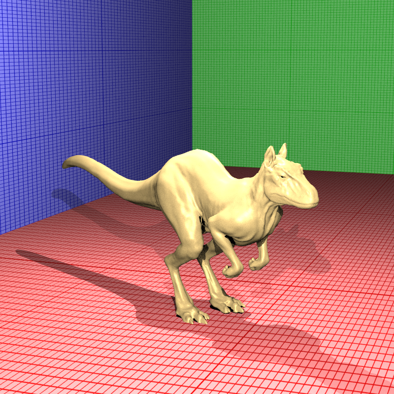
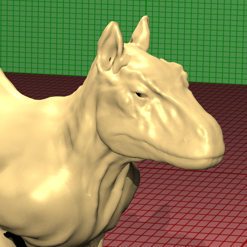
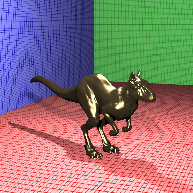
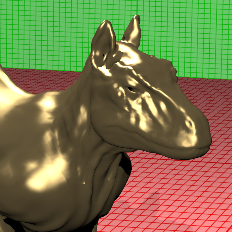
Here is a full preview of Chroma-Ray Tracer enviroment
Build instructions for Windows
Requires:
- Visual Studio(VS) 17+
- CMake 3.15.0+
Instructions
After downloading and unzipping the repo open Cmake and fill the fields:
Where is the source: unzipped/folders/directory/Chroma-RayTracer
Where to build binaries: unzipped/folders/directory/Chroma-RayTracer/build
then click configure where you will set your Visual studio version as the “Generator for this project”* and x64 as “Optional platform generator”. Also select “Use default native compilers” option if it is not already selected.
Configure then Generate.
Then open the chroma-ray-tracer.sln file generated using VS located in the ./Chroma-RayTracer/build folder.
Finally Build solution using VS.
Note: After building the project, if it fails to run due to missing .exe file try setting the location of the .exe file by:
Solution explorer -> chroma-ray-tracer -> (right click ->) properties -> General -> Output Directory ->
- if Configuration: Debug -> unzipped/folders/directory/Chroma-RayTracer/bin/Debug
- if Configuration: Release -> unzipped/folders/directory/Chroma-RayTracer/bin/Release Note2: Also do not forget to select chroma-ray-tracer as the StartUp project.
Week 1
Although I have not made any advancements regarding “Ray-tracing” I have retrofitted my old classes from my old renderer[1] to build a simple editor. This editor can;
- Load .obj files
- Render multiple lights of types:
- Point lights
- Directional lights
- Spot lights
- Support textures
- Allow basic navigation/editing over the scene
- Uses Phong Shading
Please keep in mind that footages given below are NOT ray traced in any shape or form. They are rendered using OpenGL3.
Here is a video:
Recently I started developing my RayTracer. Although I have not implemented any sort of RayTracer(yet).I retrofitted my old renderer classes and combined them with a custom ImGui UI to create a simple editor. Here is the result. I MAKE THE BUNNY DISAPPEAR in the end.MAGIC!?🎩🐇 pic.twitter.com/SqCnVzLw9Z
— Alper Ş (@stlkr_v1) February 7, 2020
Figure 1: Snapshot from Scene editor UI & Snapshot from Ray tracer window(since it uses GPU texture memory when left uninitialized it fetches some random texture).
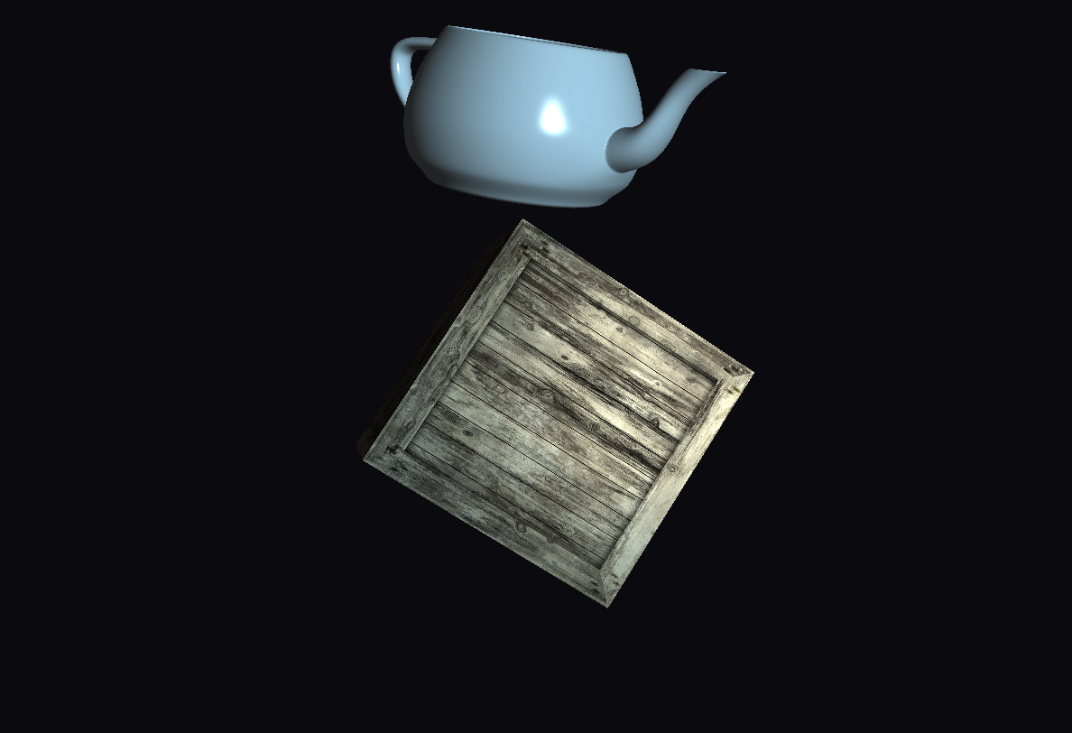
Figure 2: Example render of a Utah teapot and a crate
Week 2
Asset importer for the scene files has been completed. It simply parses the xml file to construct the scene specified by it. Figure 3 displays the scene called “simple.xml“(Provided by course instructor) as rendered in the Raster based rendering pipeline(NOT ray traced).
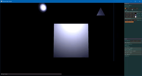
Figure 3: Raster based render of the scene from editor.
Finally, everything is set. I have started working on the Ray Tracer. Some attemps are made. Sphere-Ray intersection has been implemented and seems to be working. However rays are not allined properly. Figure 4 includes a screenshot of the sphere in the scene. It should be noted that Ray Tracer currently just casts rays and paints the pixels if they hit an object. Nothing fancy yet.

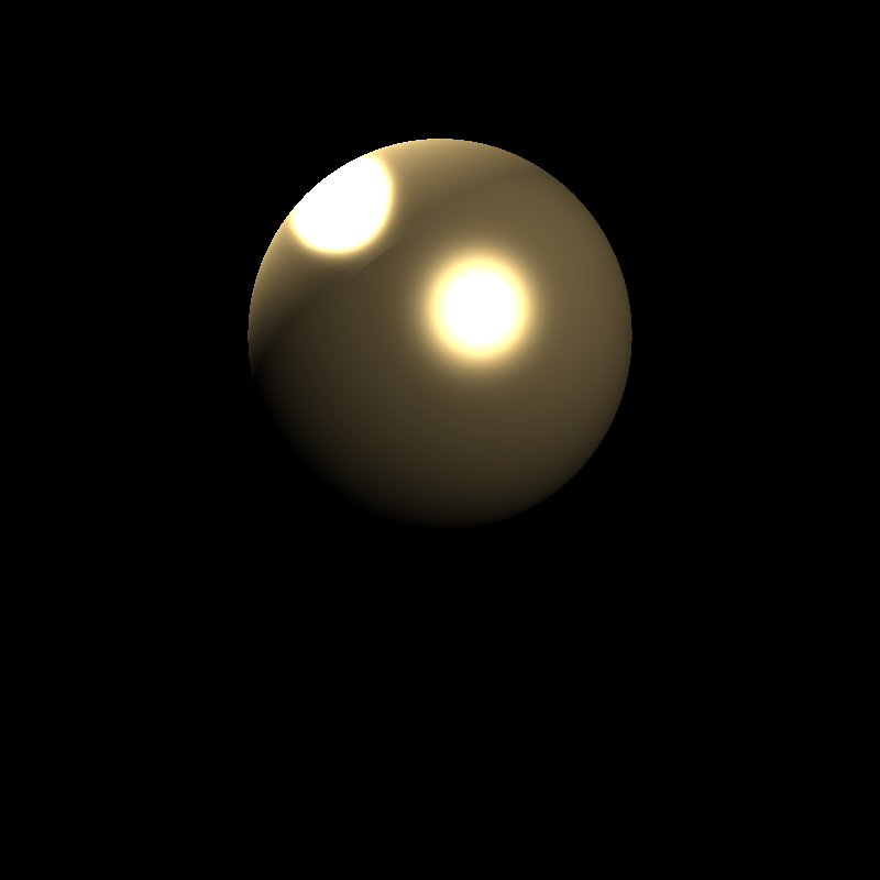
Figure 4: 300x300 image of a ray traced sphere. Failed to properly set ray directions to the near plane. No lighting calculations are made. Just hit tests.
After some fiddling with the code I have found the errors. One of the particular errors I have encountered was causing occluded objects to be rendered as if the objects that occlude them were “transparent”(see Figure 5). I quickly realised one must take the smallest t value when considering ray hits at ray direction t. After solving this problem, I was able to implement the ray tracer without shadows. Figure 6 displays spheres scene without shadows. I have implemented Möller-Trumbore’s method for ray-triangle intersections which is a efficient implementation of Cramer’s rule[2]. The introductary article and the intersection methods on the scratch a pixel website was also utilized[3]. For the sphere intersection I implemented a simple “discriminant-based” method.
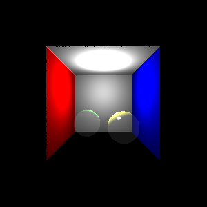
Figure 5: Failed render of the Cornell box due to dept problem.
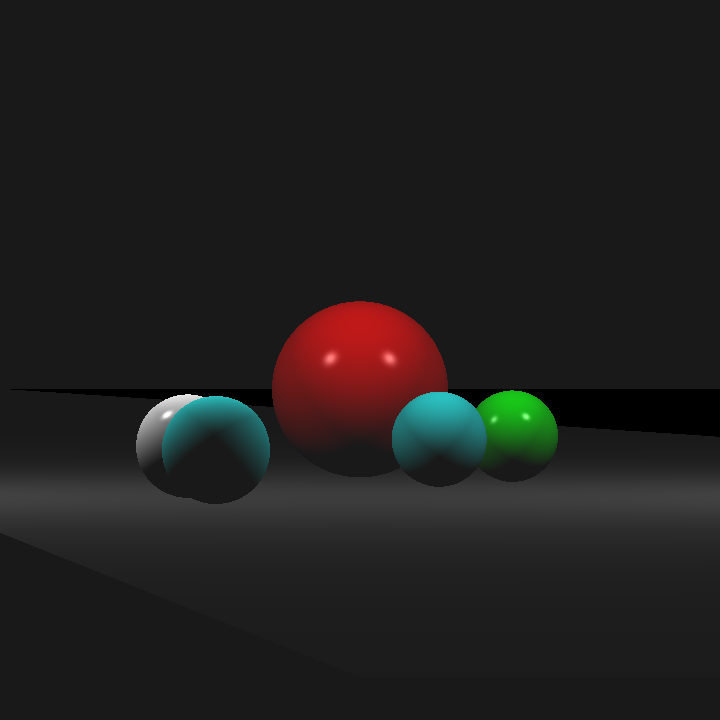
Figure 6: Shadowless render of spheres scene.
Week 3
To begin with shadows, I have implemented a loop that goes over all the scene objects to check if they occlude the light or not. I have used the same intersection methods in the week 2 to check if the rays cast from intersection point to light position intersects with another scene object. However, this part deemed it self to be very challenging since there were small intricacies.
First of those intricacies was tracking the t value in the ray equation. This was important because our shadow rays may reach to the light and keep going until they intersect an object behind the light where we mark this ray as shadowed although it is not. Figure 7 illustrates this problem. And Figure 7 displays the render failure due to this error.
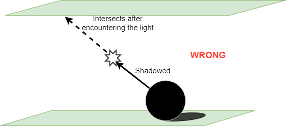
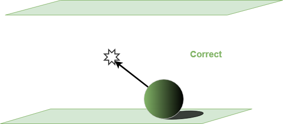
Figure 7: On left object is shadowed due to extra intersection, on right correct calculation is shown.

Figure 8: Failed render of the Cornell box due to incorrect shadowing.
Another problem I have encountered was the mistake in the Scratch a pixel’s implementation of the Möller-Trumbore method. This implementation did not returned false when t in the ray equation is negative. So a ray that has an object behind it’s origin returned true although it should not have. Of course this was not a problem for the camera rays since they did not encounter anythşng behind them yet this was causing problems when we triend to calculate shadow rays. Thats why this error went unnoticed until now(and possibly by the authors of the article [3] ). Figure 9 Demonstrates the render failure due to this problem. I have tweeted about the problem if one deems this subject interesting he can follow the link: twitter stlkr_v1’s tweet
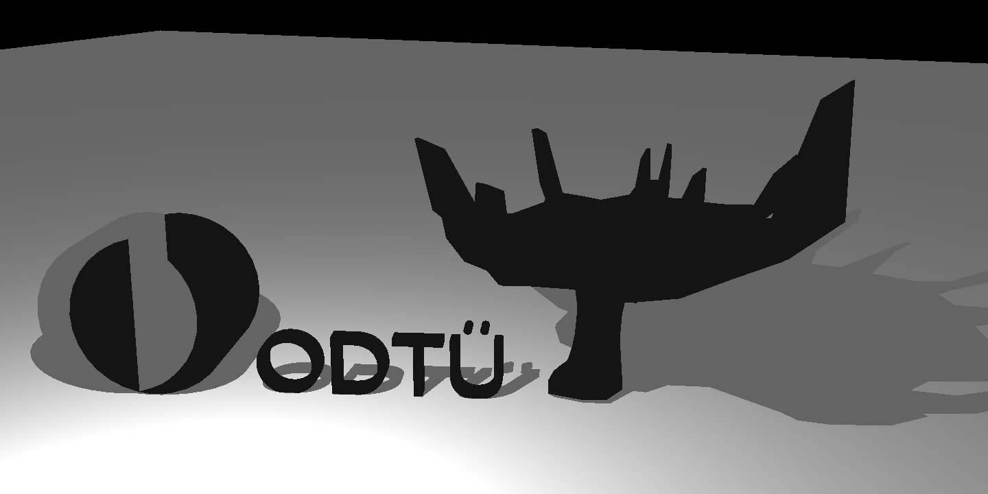
Figure 9: Render failure at the science tree scene due to negative t values for shadow rays.
To conclude interms of HW1, here are my final renders of all the scenes provided:
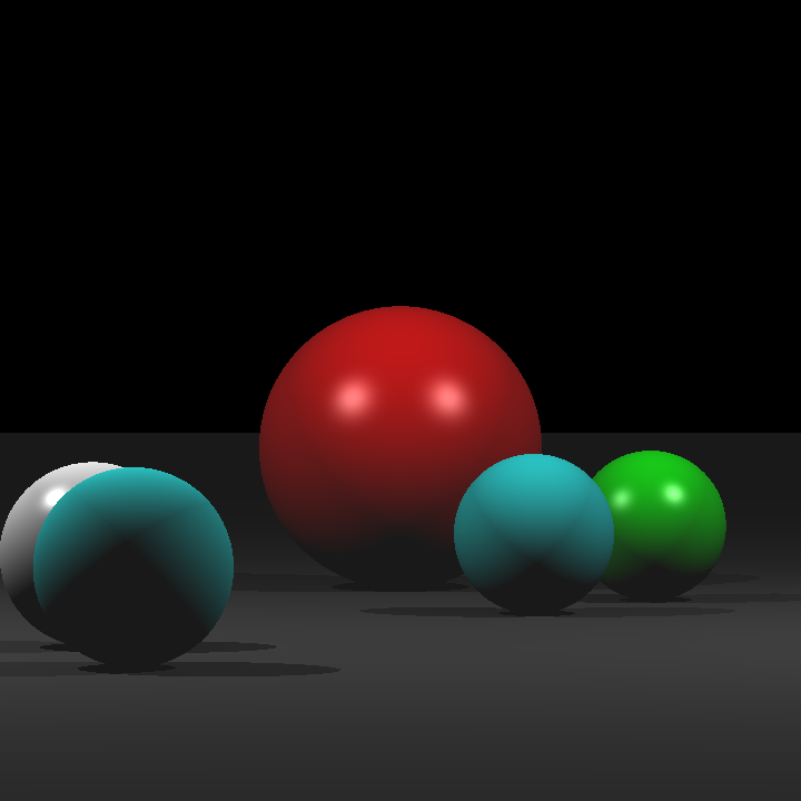
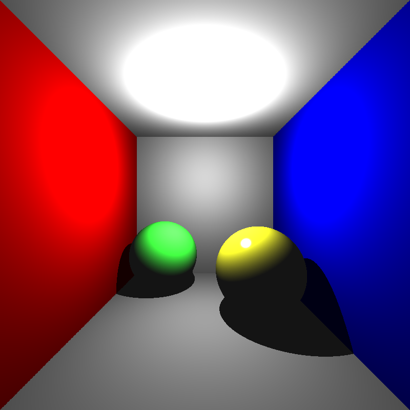
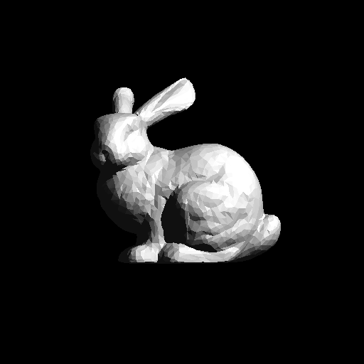
Figure 10: Final renders for HW1.
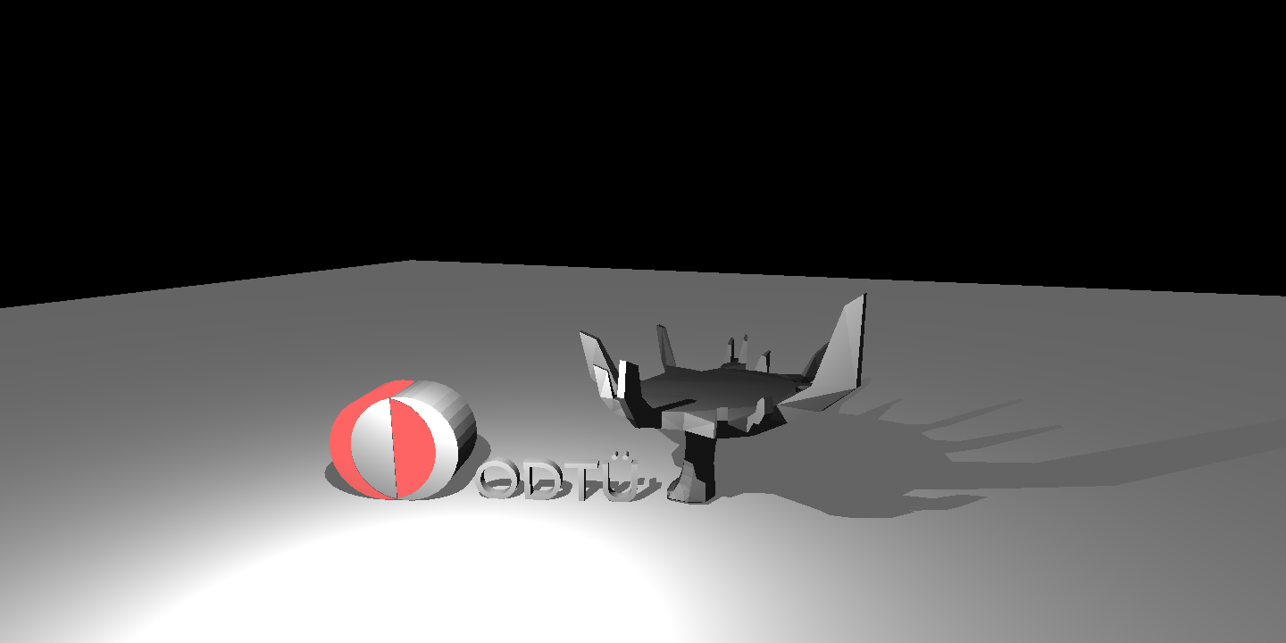
Figure 11: Final render of the ODTU “science tree” and logo. This can be considered as treason among “Bilkenters”.
This week I have managed to multi-thread the ray-tracer.Table 1 shows some statistics including thread counts.
Table 1: Scene and render statistics.
| Scene Name | # of Triangles & Spheres | Resolution | # of Treads | Render time(s) |
|---|---|---|---|---|
| Simple | 5,1 | 800x800 | 8 | 0.1071 |
| Spheres | 6,5 | 1440x720 | 8 | 0.1644 |
| Cornell Box | 10,2 | 800 x800 | 8 | 0.5071 |
| Bunny | 4968,0 | 512x512 | 8 | 13.1100 |
| Science Tree | 2240,0 | 1440x720 | 8 | 28.8958 |
Week 4
For this week, some acceleration structures have been implemented. To begin with this task, the interface for the acceleration structure has been implemented while maintaining the old classes. After that some experimentations with bounding boxes are made. After expriencing their gains and limitations. Bounding Volume Hierarchy(BVH) structure was implemented. For this task I have followed the Scratchapixel’s tutorial about acceleration structures[4].
As expected, during this process I have encountered some bugs;
- The tutorial did not consider spheres as seprate objects with different intersection geometry.
- Solved sampling points over each sphere’s surface to feed into BVH bounds.
- Nearly all meshes provided in the hw1 were “thin meshes” meaning all of their vertices lay in the same plane. This caused a major problem for BVH since properly bounding them and finding their intersection from both sides of their faces using those bounds was difficult(see Figure 12 for the render fail).
- Solved by bounding meshes with slightly larger boxes. I have also made adjustments to my mesh intersection methods since they rendered with minor backface-clipping issiues.
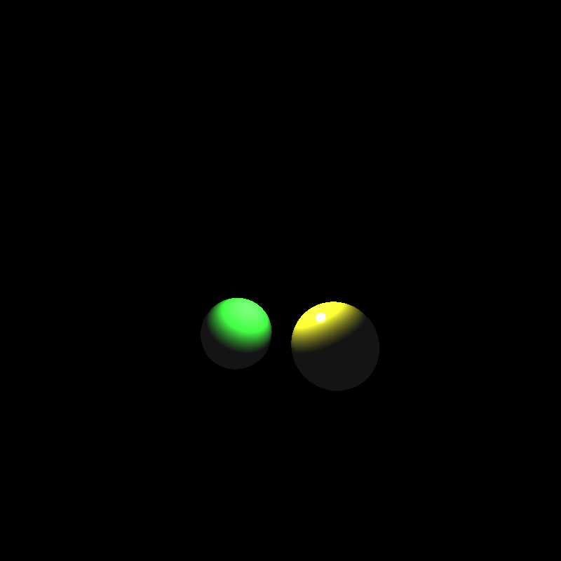
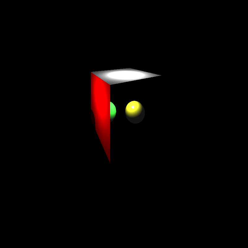
Figure 12: Cornell box scene cannot be traced with tight BVH bounds since it contains “thin meshes”.
Table 2 displays new render statistics with BVH using the scenes from hw1.
Table 2: Scene and render statistics with BVH acceleration
| Scene Name | # of Triangles & Spheres | Resolution | # of Treads | Render time(s) |
|---|---|---|---|---|
| Simple | 5,1 | 800x800 | 8 | 0.0328 |
| Spheres | 6,5 | 1440x720 | 8 | 0.1714 |
| Cornell Box | 10,2 | 800 x800 | 8 | 0.2538 |
| Bunny | 4968,0 | 512x512 | 8 | 5.8057 |
| Science Tree | 2240,0 | 1440x720 | 8 | 2.2952 |
Week 5
Implementation for a (recursive) path tracer has been completed. Now transparent and reflective objects can be rendered physically accurate. To calculate these we have considered 2 types of materials; conductors and dielectrics(and also mirrors). The programming the ray calculations for the conductors (and mirrors) were fairly easy since they only reflect the light that hits their surface. However dielectrics pose a challenge since they have many cases to handle along side with reflecions such as refractions, total internal reflections and light absorptions.
To find the amount of light emmited from the dielectric and conductor materials we use Fresnel equations along side with Snell equations to find the refraction angles[5]. We also use Beer’s Law to find light absorptions when passing through a medium.
Despide all my efforts there remains to be a small refraction error when we examine the dielectic materials. Figure 13 shows the error in the science tree scene. The problem was due to applying shading inside a medium. This is not physically correct since we cannot draw a straight line from the internal reflection/refraction point to the light source. After disabling the shading I was able to get the correct render.
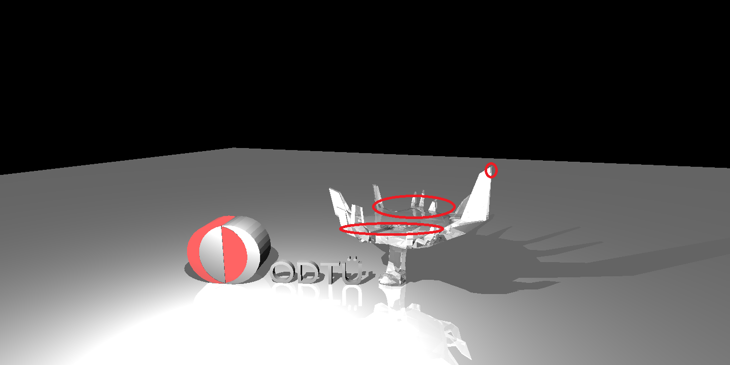
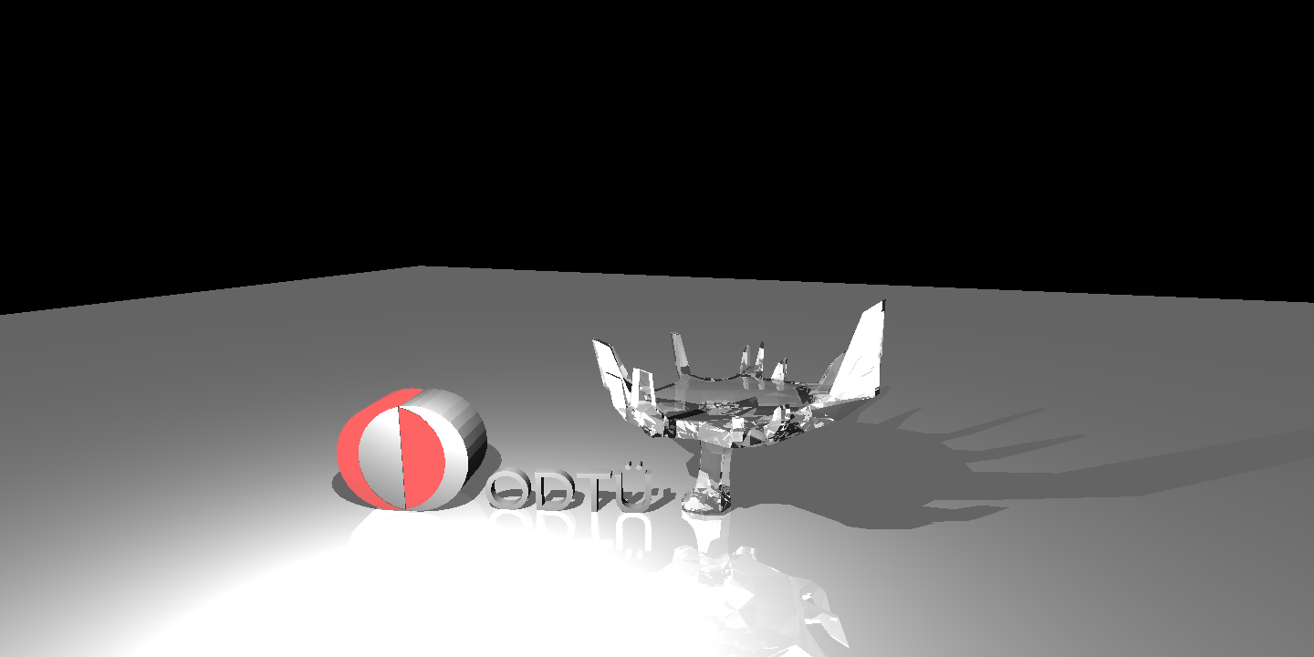
Figure 13: Left shows the failed render with missing dark refractions; right shows the correct render(courtesy of Assoc. Prof. Oğuz Akyüz).
As it turns out my previous implementation og BVH was not dividing objects in them selves but it was just dividing the scene until the bounding boxes of the objects were reached. So I had to decouple and scrap the whole acceleration structure hierarchy. Let me tell you this: “It was NOT easy!”. But I made it. I was able to imlement a BVH very similar to PBRT version. So I am using Surface Area Heuristic(SAH) to divide the scene(and objects in it!).Additionally, I was able to adapt other heuristics from PBRT[5]. After implementation all of my provided scenes were rendering faster and correctly.Except the Spheres scene that scene where I had the self collision problem of some rays. Yet this was an odd error since shadow achne was only appering on the right hemisphere of the “sphere” objects. And it was only for the shadow ray of a diffuse sphere(not a dielectric or conductor one).Figure 14 depicts the render fail. I was able to solve this by applying a lower bound threshold for t on BVH bounding box intersections.
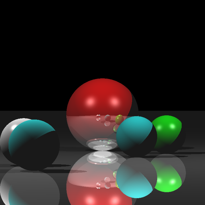
Figure 14: Incorrect shadows due to shadow rays colliding with spheres they are cast from.
To conclude interms of HW2, Figure 15 displays my final renders of all the scenes provided and Table 3 shows the render statistics for the scenes using SAH BVH:
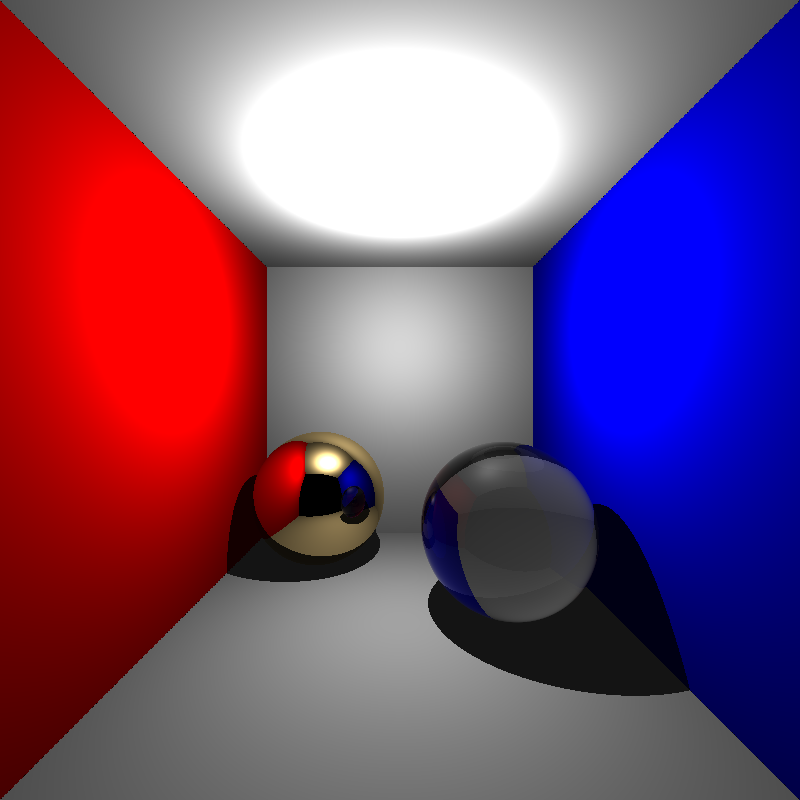
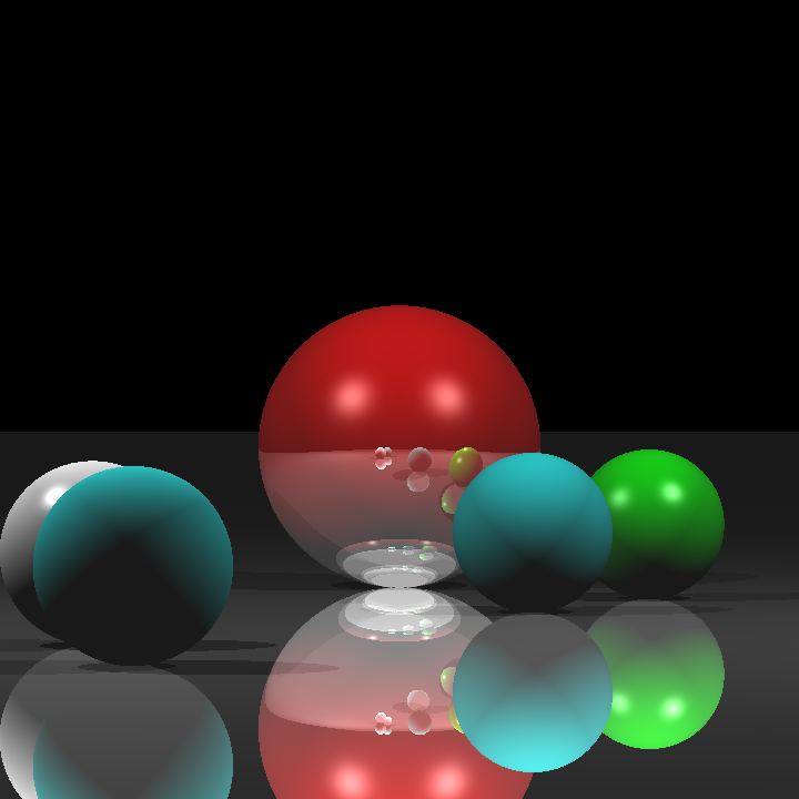
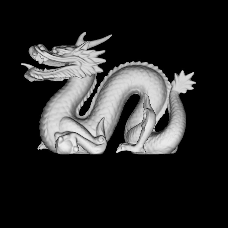
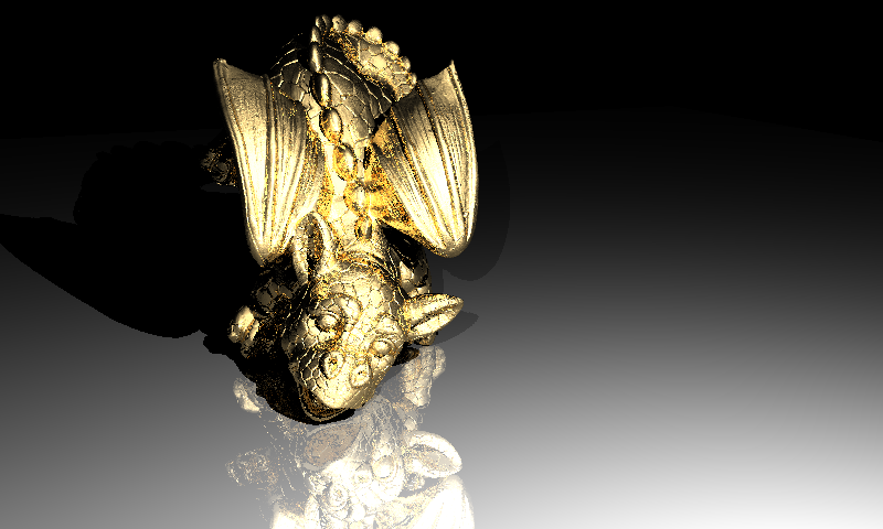
Figure 15: Final renders for HW1.
Table 3: Scene and render statistics using SAH BVH acceleration
| Scene Name | # of Triangles & Spheres | Resolution | # of Treads | Render time(s) | Recursion Depth | BVH size(MB) | # of BVH nodes |
|---|---|---|---|---|---|---|---|
| Cornell Box | 10,2 | 800x800 | 8 | 0.2201 | 6 | 0.0004 | 13 |
| Spheres | 6,5 | 720x720 | 8 | 0.1328 | 6 | 0.0003 | 11 |
| Chinese(Stanford) Dragon | 871414,2 | 800 x800 | 8 | 0.1711 | 6 | 52.5348 | 1721461 |
| Science Tree | 2240,0 | 1440x720 | 8 | 0.9363 | 6 | 0.1352 | 4431 |
| Other Dragon | 1848604,0 | 800x480 | 8 | 1.2212 | 6 | 112.8229 | 3696981 |
I have also mixed and matched some of the scene vertex data, lighting, material, etc. to make some new walpapers
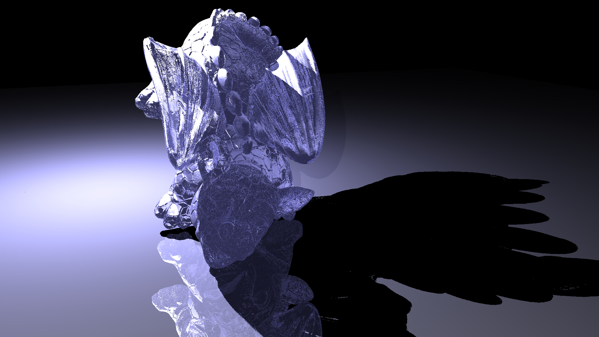
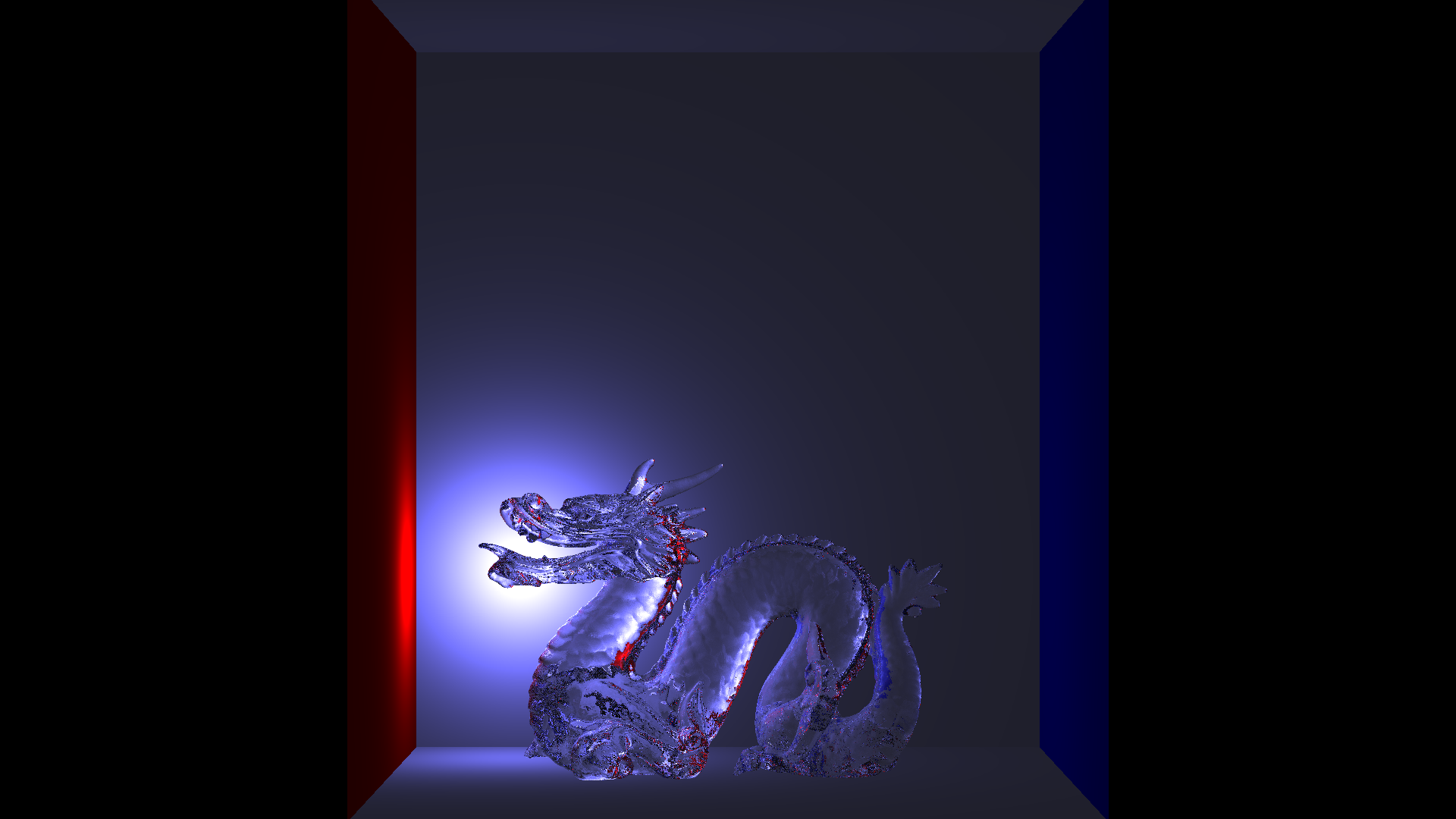 Figure 16: Additional renders of “Glass Dragon” and “Stanford Dragon in Cornell box” scenes.
Week 6
Some new GUI features are implemented:
- Material editor
- Toggleable reflections/refractions/shadows

Also material has beed made a base class from c++ struct to support proper hierarchy of fresnel materials. Material class children are:
- Mirror
- Conductor
- Dielectric
Week 7 & 8
Due to Corona virus spread development is slowed. Yet despite the chaos some new features are implemented. Most significant one of these features is Multi-Sampling. Currently Chroma Ray-tracer can Anti-Alias(AA) using Jittered Sampling Algorithm and Box filtering.
As usual C++ development is not devoid of trials and errors in the path of properly operating ray-tracer. So here are some of the bugs created and logical errors I made:
- Mis-calculation of world coordinates of samples caused rays directions to be shifted drasticly (Figure 17 a)).
- During uniform sampling random sample offsets did yield a value between 0-1 therefore it rendered a very blurry image(out-of focus)(Figure 17 b)).
- Forgot to apply filter to jittered sample. Whoops :](Figure 17 c)).

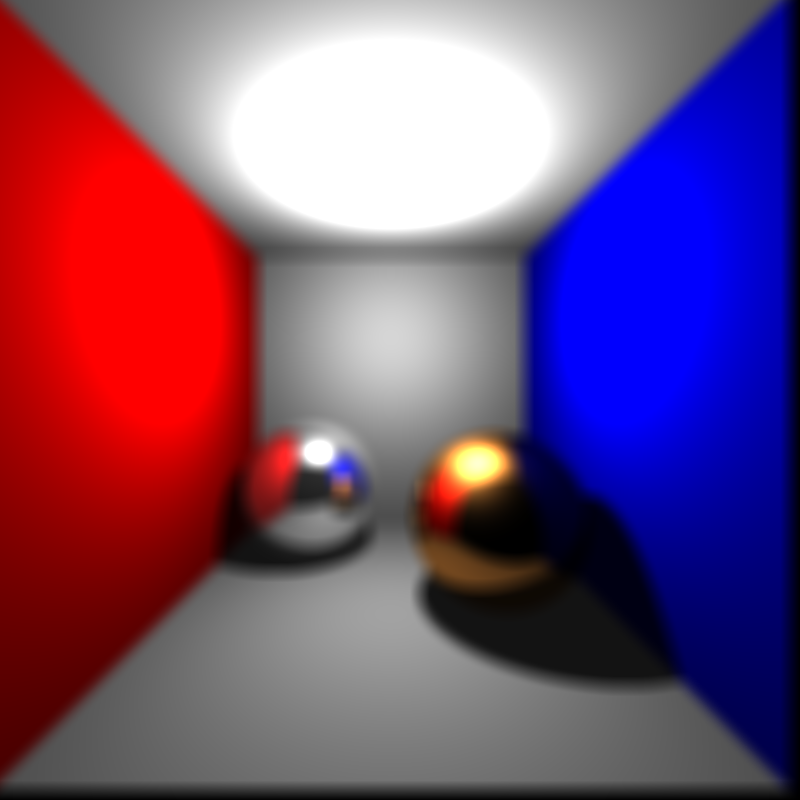
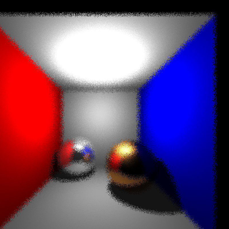
Figure 17: Render failures in the CornellBox scene due to;
a) an Error in world calculation causing shift of ray directions.
b) random offsets not being between 0-1.
c) No filtering.
After fixing and patching all the bugs it is easy to observe the effects of AA( see Figure 18). Escpecially in the areas such as wall corners or edges of objects.
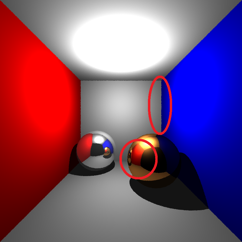
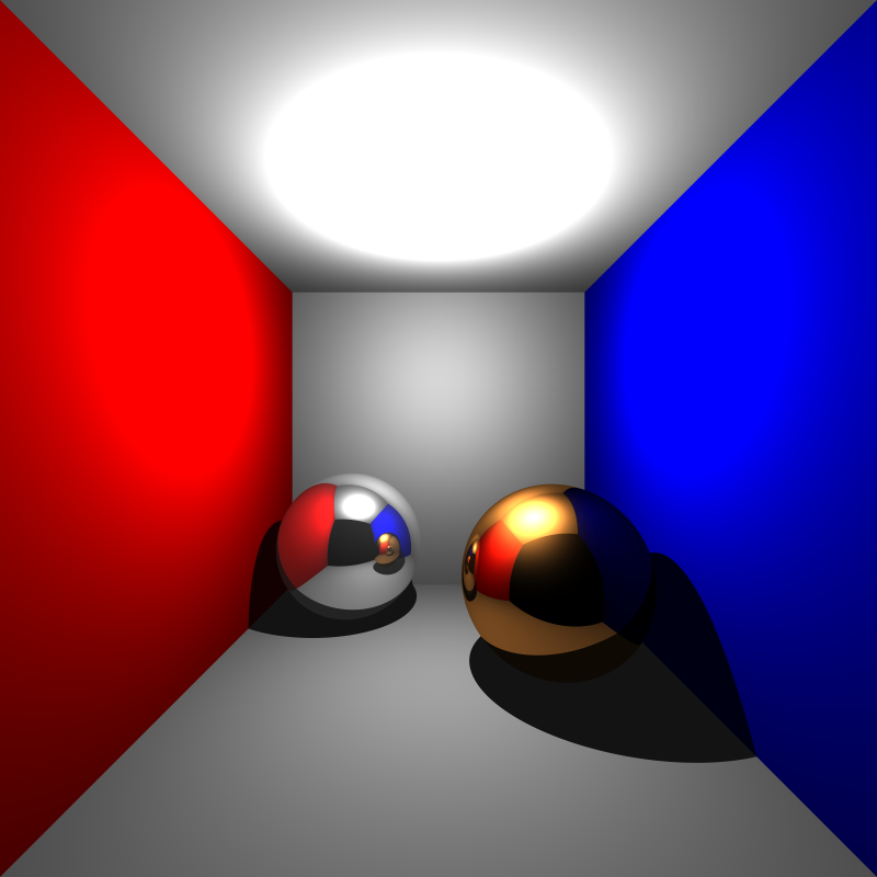
Figure 18: Cornell box scene with
a) 1 sample per pixel(no AA). b) 400 sample per pixel.
Week 9
To begin with the week, glossy reflections are implemented as desribed in the paper by Cook et. al [6]. Although it was fairly easy to achieve the desired effect there was one particular error that caused what I now call “flower” artifacts. These artifacts were caused by the random uniform sampling of the coefficients not being between -0.5,0.5. The value range initially picked was 0,1(caused flower artifacts in Figure 19). The calculation for glossy reflection ray direction can be formulated as follows:
r_glossy = normalize(r + material.roughness * (u * rand(range) + v * rand(range)));
where r is the perfect reflection direction rand() is random number between range parameter which in our case -0.5,0.5. u and v are vectors for orthonormal basis to origin of the reflection ray.
Figure 19: Cornell box scene with
a) flower artifacts due to wrong range for random sampler.
b) proper glossy reflections.
Week 10
This week transformations have been implemented. If I had to describe the process in a sentence: It was a damn tough cookie to crack. Like always there were many errors and bugs along the way. To summarize the significant ones:
- While calculating the rays in object space ray origin and direction had to be multiplied with inverse transformation matrix. What I missed out on was that the ray origin is a point where as direction is a vector. Therefore their multiplication with inverse transformation matrix should have been padded with 0 and 1 respectfully(due to homogeneous coordinates).
inverse_ray.origin = inverse_transform * vec4(ray.origin, 1.0); inverse_ray.direction = inverse_transform * vec4(ray.direction, 0.0); - Normal calculation was bit problematic due to sphere objects. The problem turns out to be the center point provided in the scene files. Since Chroma RT was using centers as seprate fields rather than translation it needs to be transformed when calculating normal of the spheres using the transformation matrix.
transformed_center = transform * vec4(center, 1.0); normal = normalize(inverse_transpose_transform_mat * (intersection_point - transformed_center)); - Also BVH bound calculations for the spheres contained logical mistakes. Mistake was after applying transformations to bounds, bounds had to be rebounded since the tranformed bounds may not be axis-alligned (see Figure 20).
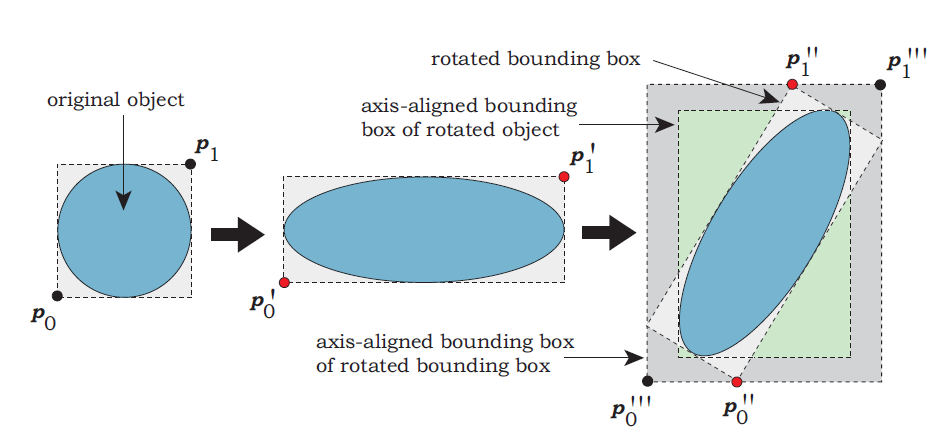
Figure 20: The axis-aligned bounding box of the rotated bounding box is larger than the
axis-aligned bounding box of the rotated object [7].
Many solutions to these bugs came from Kevin Suffern’s “Ray Tracing from the Ground Up” book [7].
Depth of field(DoF) effects were also implemented this week. Although image plane and focal point calculations were little confusing at start internet and Suffern’s book helped a lot [7]. Side note on my implementation of DoF rather than sampling on a unit square for lens point Chroma does the proper thing and samples on a unit disk although the difference is minimal(so does the effort put into it).
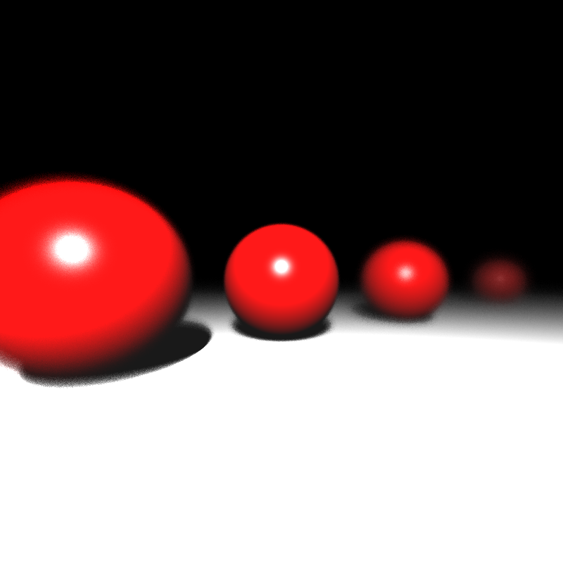
Figure 21: Sphere transformations and depth of field effect demonstrated in an example scene.
While deadline closes in I was able to patch up some errors and implement instancing and motion blur effect(for translation only). One of the difficulties faced during the development of motion blur was BVH integration. Since BVH sets up tight bounds for shapes when the Intersect for that particular object is called it will only be for it’s still position and inverse transforming the rays will only make the look of the object noisier/transparent. Figure 22 illustrates this problem in 2D.
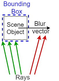
Figure 22: Diagram on the left displays the mistakenly tight bounded BVH bounding box where the rays that are supposed to give the blur effect fails to intersect the box. Diagram on the right displays the correct bounding box construction.
To top it off:
- Some optimizations are made regarding memory efficiency(using stack objects rather than heap).
- Implemented a async. progress bar printed on to console(can be seen in the Introduction previews) since successive prints effected the cpu efficiency.
- Smooth shading option for meshes.
Figure 23 shows the final renders of HW3 and Table 4 shows the render statistics for those scenes.
![]()
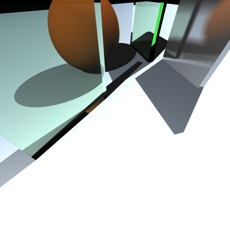

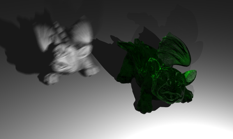
Figure 23: Final renders for HW3.
Table 4: Scene and render statistics for HW3 scenes.
| Scene Name | # of Triangles & Spheres | Resolution & Sample per pixel | # of Treads | Render time(s) | Recursion Depth | BVH size(MB) | # of BVH nodes |
|---|---|---|---|---|---|---|---|
| Simple Transform | 3,1 | 800x800,1 | 8 | 0.8255 | 1 | 0.0002 | 7 |
| Spheres DoF | 2,4 | 800x800,100 | 8 | 95.8729 | 6 | 0.0003 | 9 |
| Cornell Box Brushed Metal | 10,2 | 800 x800,400 | 8 | 515.727 | 3 | 0.0004 | 14 |
| Cornell Box Dynamic Boxes | 36,0 | 750x600,900 | 8 | 845.3153 | 4 | 0.0012 | 39 |
| Metal Glass Plates | 38,1 | 800x800,36 | 8 | 202.5724 | 6 | 0.0014 | 47 |
| Tap | 50316,0 | 1000x1000,100 | 8 | 353.9330 | 6 | 2.8705 | 94061 |
| Dynamic Dragon | 3697206,0 | 800x480,100 | 8 | 16752.1317 | 6 | 225.6457 | 7393959 |
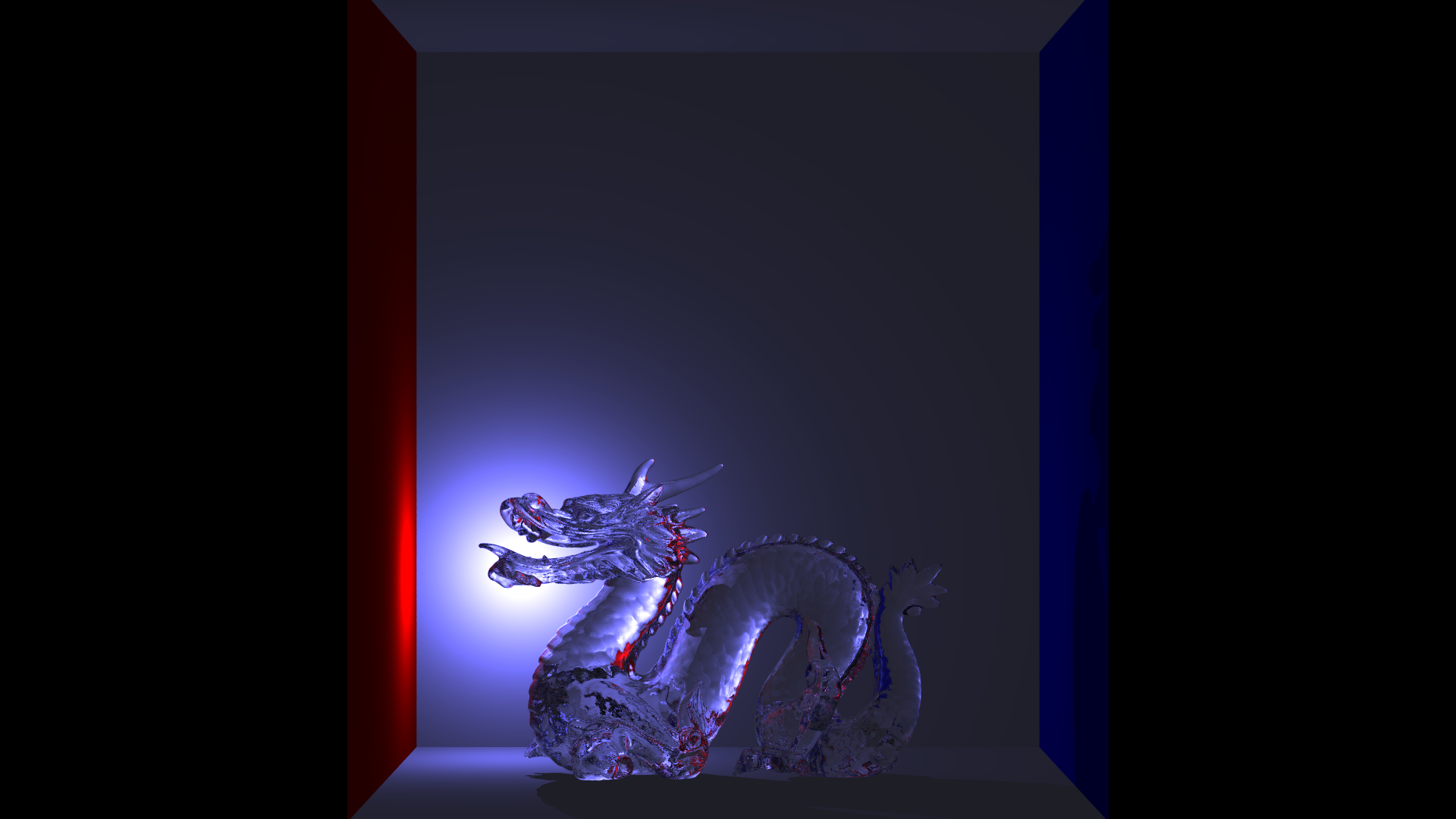
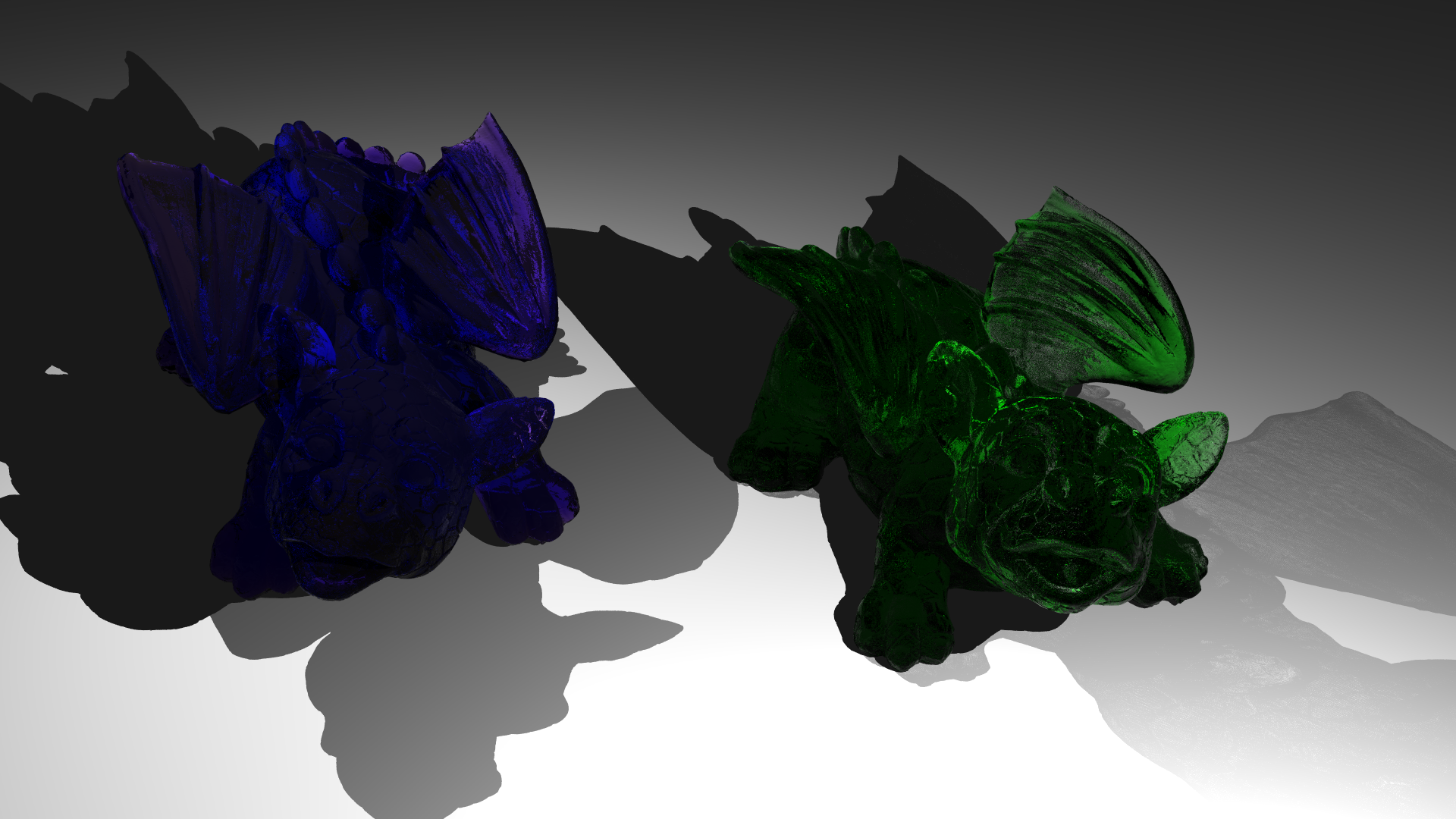
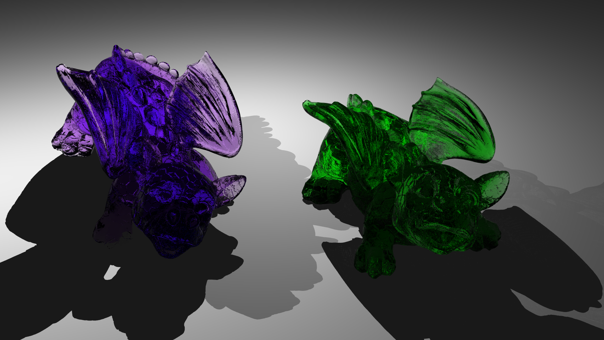
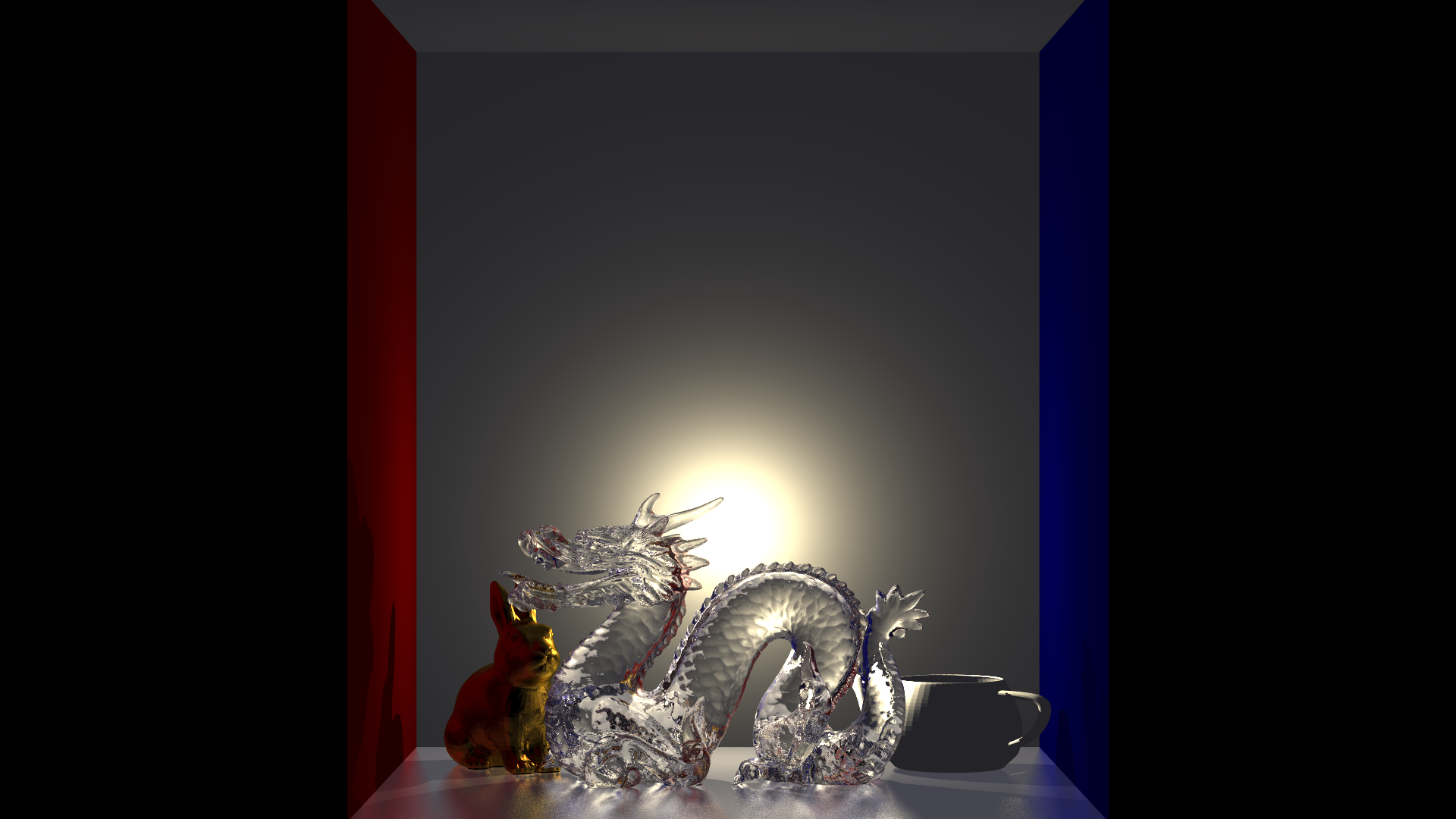
Figure 24: Additional renders.
Week 11 & 12
These weeks were focused on development of texture mapping along side with normal and bump maps. Perlin noise was also implemented. Of course during this process there were some significant mistakes made.
For the triangles texture coordinates are calculated using the barycentric coordinates of the hit point. To calculate the texture value we require U,V values for the position ray hits. However this value is an weighted average of triangle corner UVs where weights are barycentric coordinates. The problem I faced was dues to my own laziness. Since I did not wanted to calculate which corner gets which barycentric coordinate I forced my way through trial&error. As it turns out correct combination for my implementation was 1,2,0 as follows:
u * corner_uv[1] + v * corner_uv[2] + (1-u-v) * corner_uv[0]
Yet along the way such fun render fails are achieved(see Figure 25).

Figure 25: Left render failure due to wrong calculation of barycentric coordiantes, right correct rendering.
During the implementation of Perlin noise on sphere I had similar difficulties. As it turns out calculation of tangent space vectors was off and due to that I get pretty cool render fails. One can see those in Figure 26.
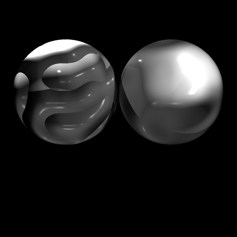
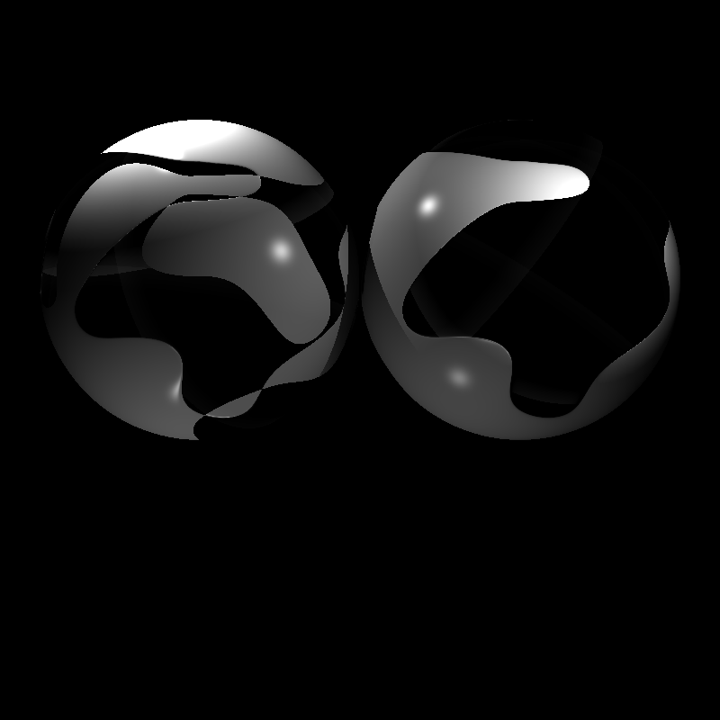
Figure 26: Render fails due to wrong calculation of tangent space for perlin bump mapping on sphere.
Lastly I figured out that Perlin weighting function should only take positive values between 0-1. Yet this was not the case in the instructors notes. However this minor error was quickly corrected after looking up Ken Perlin’s paper [8]. During this process I got and interesting artifact I like to call “Pervin Noise” (See Figure 27).
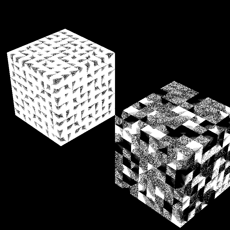
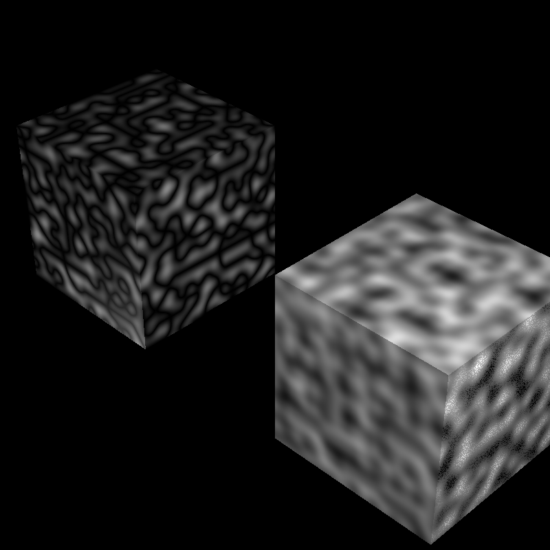
Figure 27: Left, Perlin Noise with negative values fed into weight function. Right, correct render of that scene.
After fixing these issues most of the process was straight forward. During one of my renders I got an interesting render using Perlin Noise. On one cube’s side a “dude” poped up with sun glasses and a cowboy hat. This can be seen in Figure 28.
I tweeted this image to check if I am going insane or not due to quarantine. Peter Shirley and many computer graphics enthusiasts took an interest to this image and saw the same dude thus proving that I was still sane.
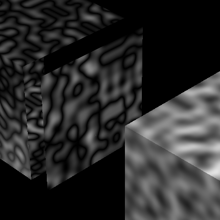
Figure 28: Perlin noise dude!
To conclude here are this weeks renders:
![]()
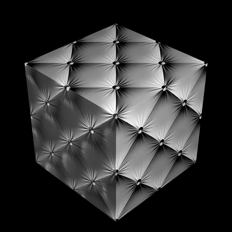
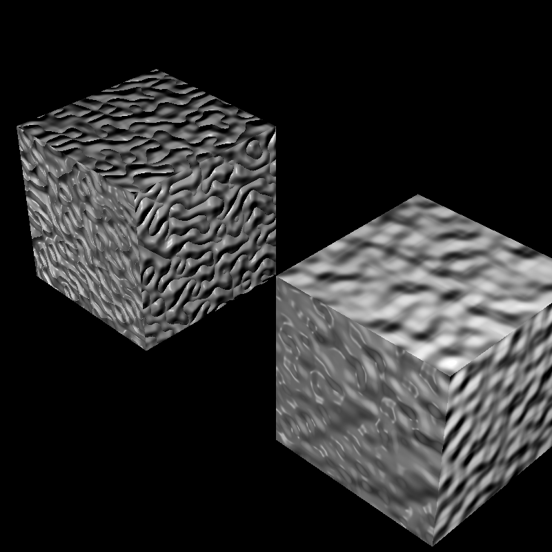
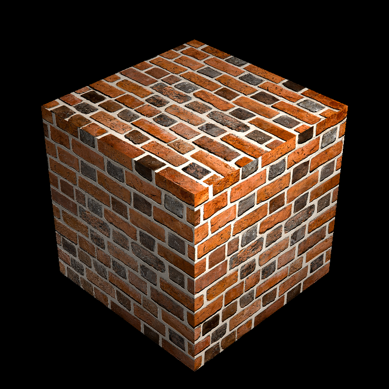
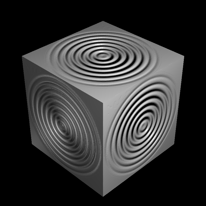
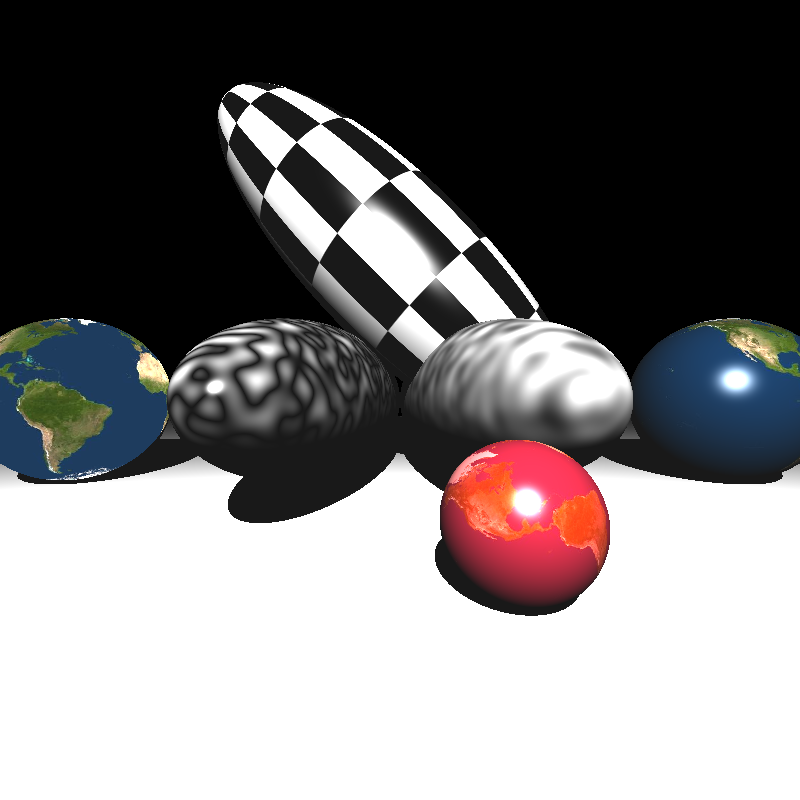
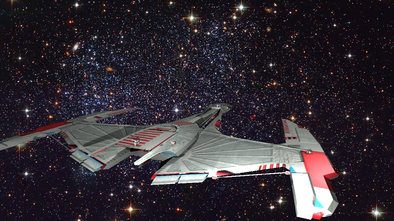
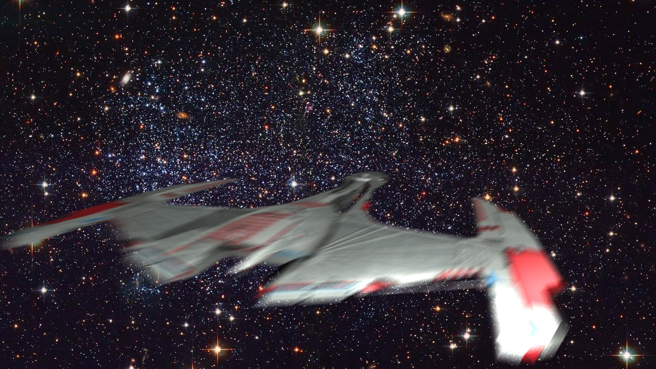
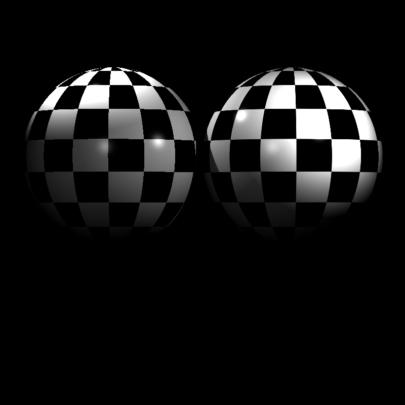
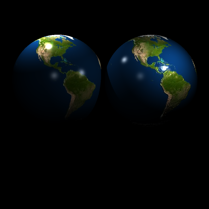
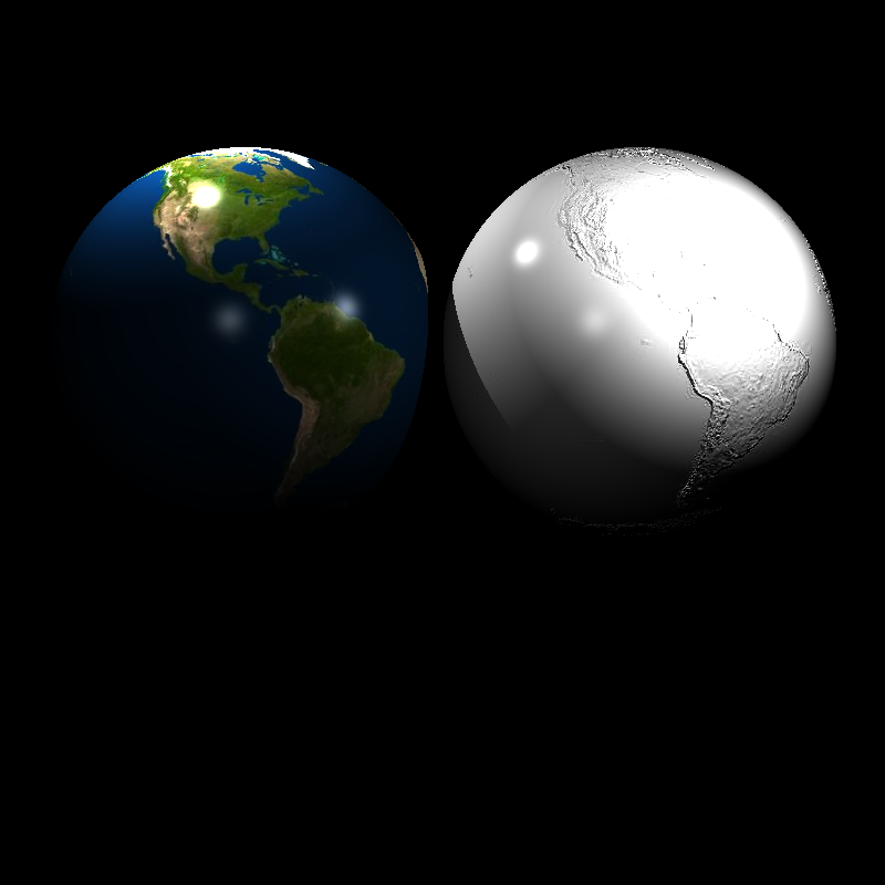
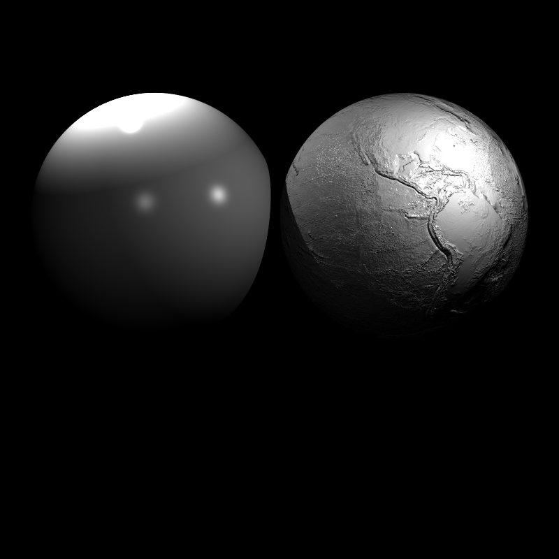
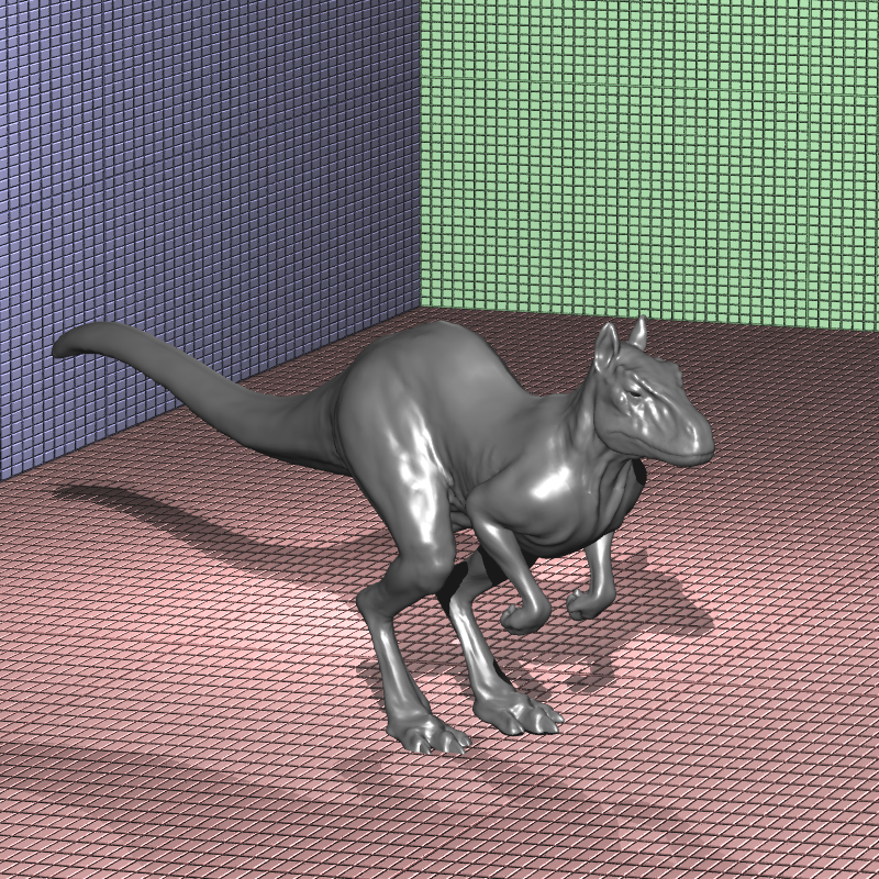
Figure 29: HW4 renders.
Also I prepared a animation that demostrates the spatial location based noise property of Perlin noise. One can observe the patterns staying still while spheres move down in y axis(Figure 30).
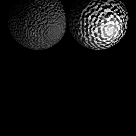
Figure 30: Perlin noise animation.
Weeks 13 & 14
These weeks were particularly difficult. I had to submit many other projects thus leaving little to no time to Chroma. However luckily I had the chance to use my late submission days(First time I used any sort of late submission in my entire academic life). All the business aside this weeks assignment was particularly difficult due to HDR imaging subjects and them being particularly not very interesting to me.
To begin with this weeks development process it was expected from us to implement the global tone mapping operator from Reinhard et al. paper [9]. Along side with some advanced lighting techniques:
- PointLight
- DirectionalLight
- SpotLight
- AreaLight
- EnvironmentLight
The implementation process of Chroma 1.14 stared with HDR imaging which required both read and write support of .exr files. Oğur course instructor recommended us the OpenEXR[10] library for this functionality however as for all C/C++ libraries it’s setup felt very complicated and tedious (except header only libraries). Given the time-constraints and the README note that says “setting up OpenEXR for VS is not for faint of hearted” let me to simpler option: tinyEXR[11]. After setting up libraries I wasted 2 days on implementing the global tone mapping operator of Reinhard et al. paper [9]. However all I ended up with was all black images so I went to forums of the course to ask about the operator. Yet some people already have asked it and they were waiting for a reply so I left it as is and went on with the advanced lighting types which I already knew some of and took more of my interest in comparison to HDR imaging.
As I mentioned before I have retrofitted my old Chroma Engine OpenGL Abstractions to Chroma Ray Tracer for preview renderer. Which also included spot and directional lights in addition to point lights. Yet since OpenGl uses a simpler interpretation of data flow these data structures were in the form of C++ structs. Therefore first thing made was to create proper Abstract Light Class:
class Light
{
public:
  //... preview renderer properties...
  vec3 Intensity;
  virtual vec3 IlliumitantionAt(...);
}
One of the key things to notice here is that terminalogy intensity here is abuse of notation however this is also very similar to how PBRT defined their Light abstract class [5]. The second thing is “IlliumitantionAt” function which calculates shading without the shadow calculation(very tightly coupled with ray tracer class). After implementing classes for all five light types I also connected them to my old forward rendering pipeline. It still produces good results in simple scenes it comes very close in many of them. Figure 31 shows forward rendered and ray traced look for the spot light dragon scene. Unfournanetly, Environmental and area lights are insivible in forward renderer thus the do not show up or effect any preview renders for now.
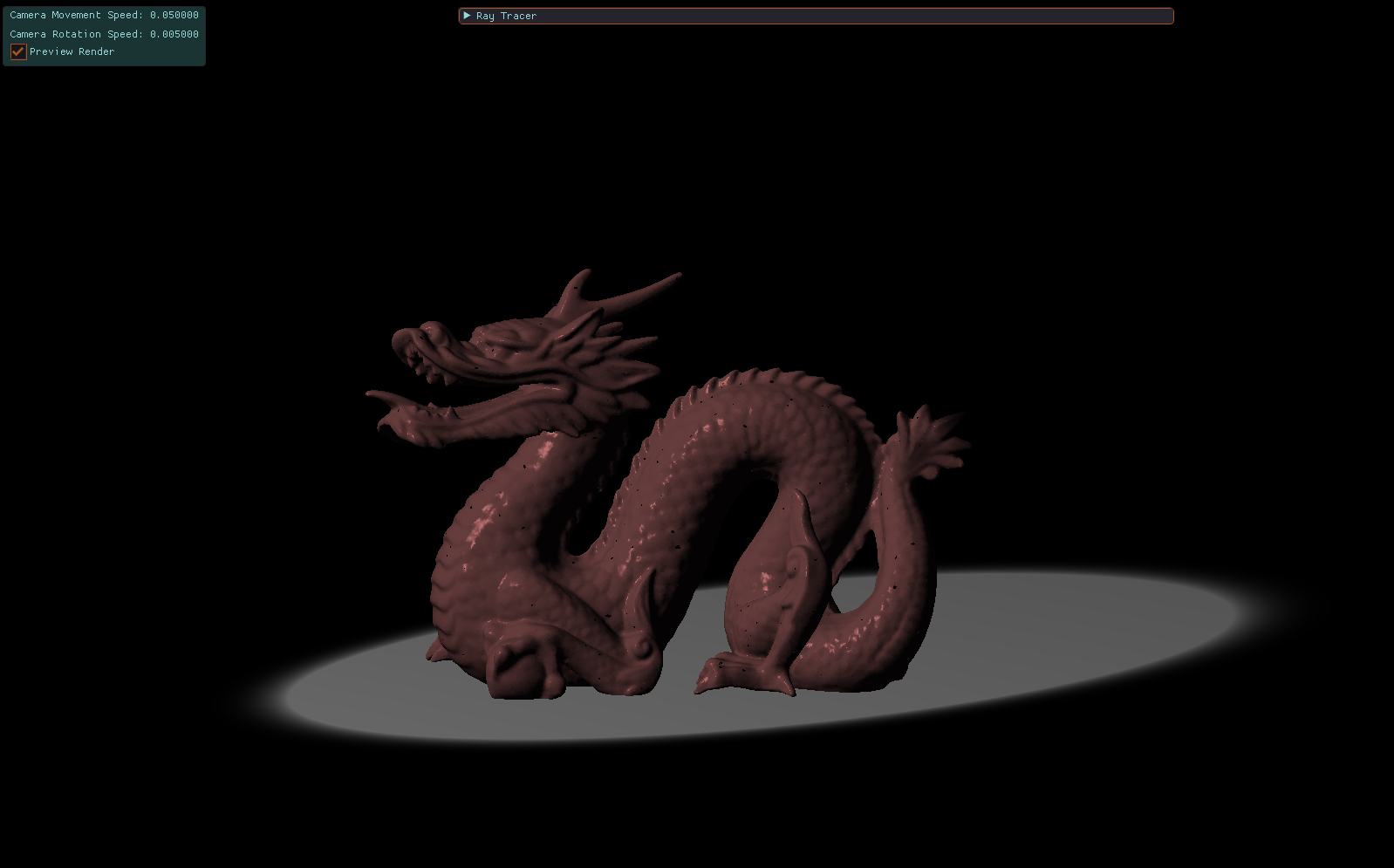
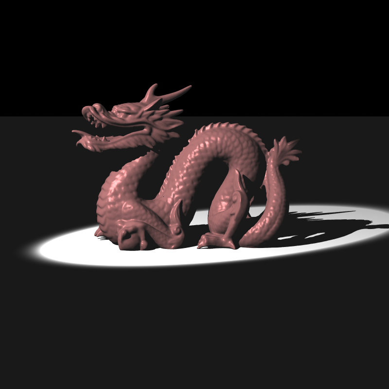
Figure 31: Forward rendered and ray traced look for the Spotlight Dragon scene.
Area Lights were particularly tricky since random number generation in C++ is not thread safe and caused many noisy outputs with comparison to reference render. Figure 32: shows reference image and my render with same number of sampling side by side.

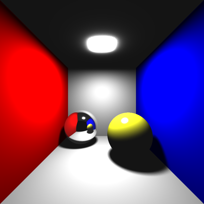
Figure 32: Left my render with 100 samples, right reference image with 100 samples.
After experimenting with various factors such as making mersenne twister engine of C++ static thread local, reading all the blogs, asking in the forums, and calling a C++ expert of friend of mine for help I found no solution to my noise problem. It is not a race condition like Bahadır points out or a safe-threadness like Serdar points out in the blogs because even the single threaded outputs are equally noisy. I also tried perturbating the light sampling points in the direction of normals and also in the direction of light vector(-intersection_point + light_position). Yet I have increased my sampling rate to 289 samples per pixel and I got very decent results(see Figure 33).

Figure 33: Cornell box area light scene with 289 samples per pixel.
After completing these I went back to HDR imaging and texturing. After reading the answers given in the forums and the paper by [9] couple hundred times. I found some crucial mistakes I made during tone maping. Most important being in order to calculate L_white one needs to find the percentage of the luminance that is specified by the parameters to put the value in the eq.3. What I did initially was using Luminances calculated from bare pixels and sorting them to find L_white. This was obviously wrong after which made it self apparent to me when I read Eda Nur’s blog. The correct thing needs to be done is sorting the L(x,y) values calculated by eq.2 of the TMO by [9].
Yet all this progress still reproduced all black images. I went down to paper and examined formulas again expecaially eq.1 since it throwed suspiciously small values. I was going to ask if there is something wrong with the formulas yet Ahmet Hocam had already found the typo and informed us that the Eq. 1 should be:
exp( 1/N * Sum_xy(delta + log(L_w(x,y))))
rather than:
1/N * exp(Sum_xy(delta + log(L_w(x,y))))
Of course knowing that Peter Shirley was among the writers. I tweeted him about this typo. He kindly replied and confirmed the error. I believe he will apply for the errata procedure to fix the typo. Of course pointing this error out felt risky to me since paper was from 2002.
Here are some render fails:
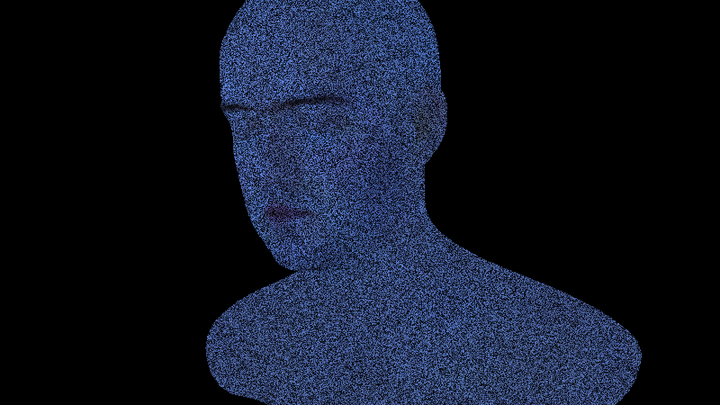
Figure 34: The new blue man group member(can only play wind instruments) and the LSD Tone Mapping operator.
Without further ado, here are this weeks renders:
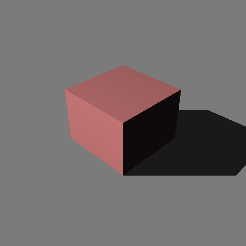
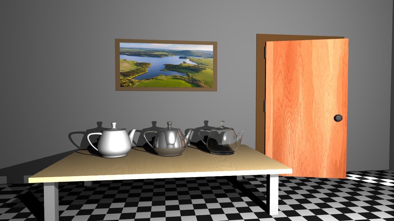
Figure 35: HW5 final renders. Cornellbox_area scene is swapped with 289 sampled version since it looks better. Veach Ajar scene camera position is maully adjusted*.
Note*: I do not know why but some scenes with lookAt cameras gives slightly different outputs in terms of camera location or sometimes aspect ratios. This might be due to floating point precision or diffetent Image Plane interpretations. Veach Ajar is one of those scenes where I had the advantage of having interactive editor camera to move around forward rendered scene to find the closest spot on the reference image. Basicly I had to back up a bit to make the FOV cover the procedurally generated checkerboard texture.
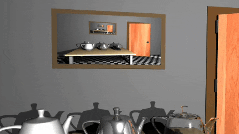
Figure 36: Veach Ajar scene infinite animation.
My API is a mess right now I will be focusing on that before the next assignment hits.
Weeks 15 & 16
This week was focused on bidirectional reflectance distribution function(BRDF) materials. The implementations included:
- Phong
- Blinn-Phong(default)
- Modified Phong
- Modified Blinn-Phong
- Torrance-Sparrow[12]
The Phong and Blinn phong was fairly easy to implement(since I have previously written GLSL shaders for them). Modified versions included energy conservation/normalization factors. Understanding the derivations was the difficult part for those BRDFS. But the trickiest among them all was Torrance-Sparrow approach. Since it is essentially a micro-faced based approach some complications were present.
The most significant problem faced during implementation was the architecture. My implementation of BRDF was implemented as a Material field. A pointer to the abstract class BRDF is present and that class holds the exponent value for the shading(this value was previously present as a field in the Material class). Since Fresnell calculation was required for Torrance-Sparrow BRDF the GetFr() function for the materials were implemented inside the Material class this caused some problems. Yet solution was apperant after close inspection of the XML scene files. It seems like our instructor came up with the smart idea to put the properties needed for fresnel value calculation to regular(typless) material fields for such BRDFs. These properties are usually present when the material is not a typeless material but a Conductor/Mirror/Dielectric. Existance of these fields allowed my architecture to have those values in TorranceSparrow class as fields. Thus giving me the this weeks renders in Figure 36.


Left with some spare time I made some adjusments to better my architecture in terms of both maintainability and efficientcy. Firstly I changed Light abstract class to have two functions instead of one giant CalculateIllumination. Those functions are SampleLightDirection and CalculateRadiance. By doing so I made the shading code a bit dity and removed redundant parameter copying operations between IntersectionData, Material, Light classes. BRDF abstract class has two virtual functions namely they are CalculateDiffuse and CalculateSpecular these private functions are called from the friend class Material’s Shade function then this shaded value is returned to IntersectionData class Shade function where it multiplies the float value with light radiance after handling the texturing business.
I was also able to beautify the Editor Code by writing an virtual ImGuiDrawable class which is implemented by all scene components that can be adjusted by the interactive inspector(cameras, sceneobjects, lights). This class has one virtual method DrawGui. Which specifies how their parameters can be ineracted by the Editor GUI. I also made some color codings and simple UI changes to make somewhat a uniform looking GUI. I also selected new colors for the UI headers of the some inspectable scene components.
Brief Project Discussion: Fast Tetrahedral Mesh Traversal for Ray Tracing
In this section is dedicated to a brief discussion on my research at Bilkent University which is correlated with the course topic.
So we know about BVH, kd-tree, Octree… as acceleration structures. Tetrehedral Meshes can also be used as spacially subdividing acceleration struture. The idea is simply filling the empty space in the scenes with tetrahedrons then tracing the rays through the tetrahedrons using ray connectivity and neighbourhood information of tetrahedrons. Figure 37 demonstrates how mesh is set up and rays are traced[13].
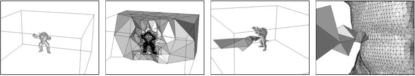
Figure 37: Accelerating ray tracing using constrained tetrahedralizations. (left to right) A scene consisting of the Armadillo model; A tetrahedralization of space that respects the geometry of the scene; A ray is traced through the tetrahedralization; A constrained face is hit[13].
Our research at Bilkent focuses on the compaction and efficiency aspect. My work specificly is on GPU kernels and efficiency on CUDA cores.
Some pros and cons of this approach:
- Can support limited deformation without reconstruction.
- Instead of full reconstruction partial reconstruction for mesh deformation and Level-of-detail(LoD) meshes can be applied.
- Very similar to grid data structure it self is highly localized so better suited for GPU application where as BVH or Kd-tree appoaches require a tree and a stack to maintain the parallelization.
- If quality Delenuay Tetrahedralization is applied Teapot-in-a-stadium problem does not occur.
- Takes more memory than any other approach.
- Takes too long to construct.
- Does not handle intersection geomtery well.
I made detailed video about my research and the method which gives more in depth information about the Tetmesh acceleration structure.
The data structure assumes 3 arrays:
- Vertex list of tetrahedral mesh
- Tetrahedron list
- Mesh/scene object list
Each tetrahedron struct is 32 bytes long:
- 3 vertex indices
- xor sum of vertex indices to find the unshared vertex during traversal.
- 4 neigbour tetrahedron pointers.
Keep in mind that this representation can be further compacted down to 20 and 16 bytes. We call them TetMesh32, TetMesh20 and TetMesh16 respectfully [14]. Although I wont be able to share too much of our “latest results” I have provided TetMesh32’s performance comparison with respect to kd-tree and BVH in Figure 38
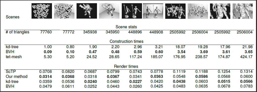
Figure 38: Construction and render times for different methods [14].
NOTE: In the video I mistakenly say render times are microseconds. They are actually seconds.
In my video I also talk about the benefits of Hilbert sorting tetrahedra in memory to achive better results. One can look at Figure 39 for effects of sorting for the scenes provided in Figure 38.
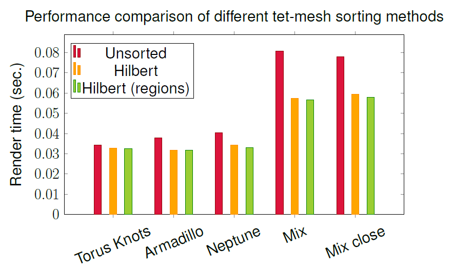
Figure 39: Render time comparison for unsorted vs. sorted tet-mesh data.
I can finally demonstrate some preliminary results concerning render times for various tet-mesh compaction schemes namely TetMesh32, TetMesh20, TetMesh16 and TetMeshScTP(original method described by Lagae et al. [13]). As it turns out in general TetMesh20 is faster in the CPU where as TetMesh16 is faster in the GPU. This is due to extra operations required to unpack TetMesh16 during traversal(see Figure 40). With enough number of cores GPU can handle this operation in bulks where as in CPU very limited number of cores creates an instruction level bottle neck for TetMesh16 rather than a memory bottleneck. Keep in mind that the figures provided measures render times. This includes ray initialization(in CPU), traversal and draw times for CPU; ray initialization(in GPU), traversal, intersection data copy time and draw times for GPU
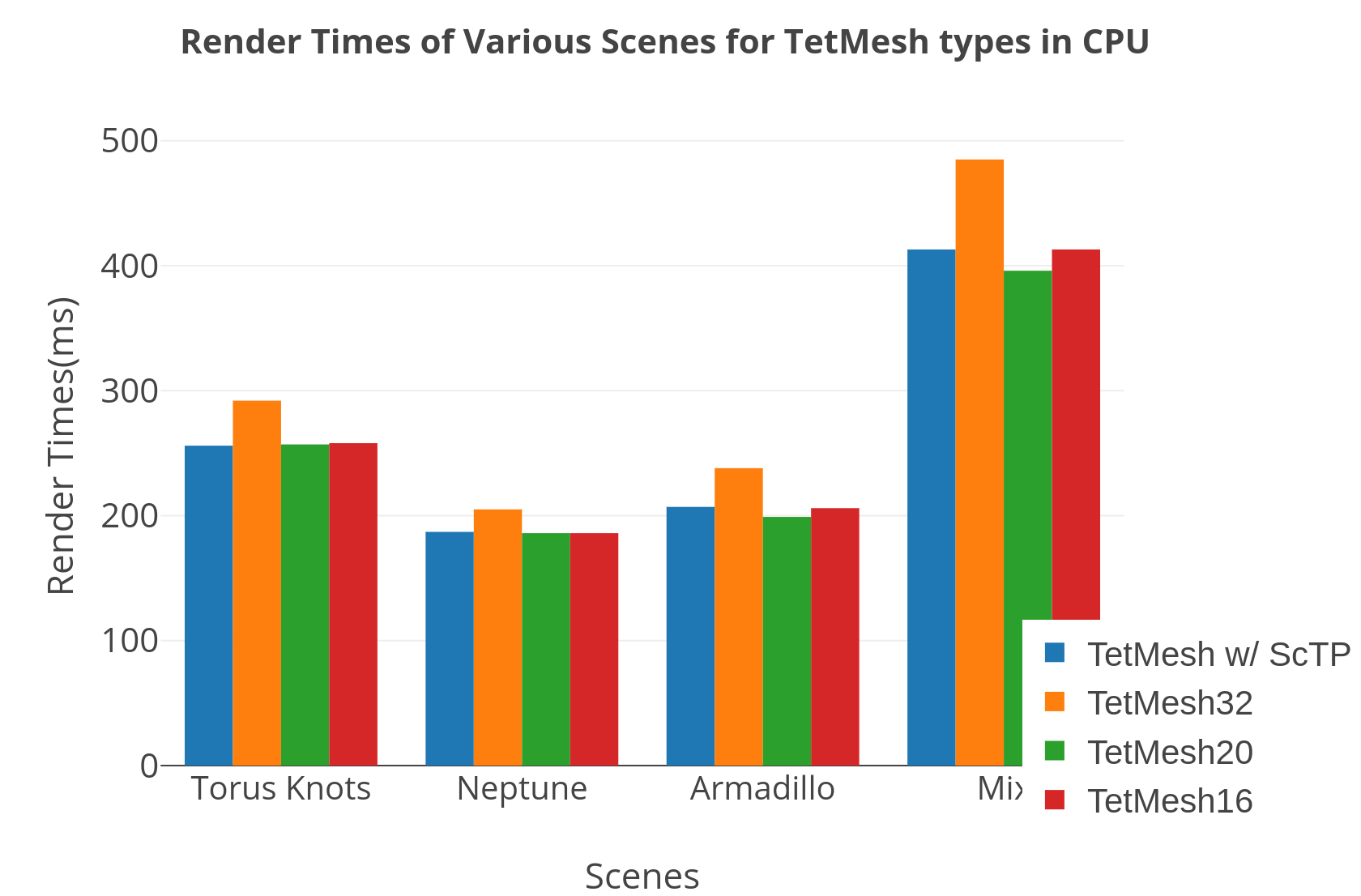
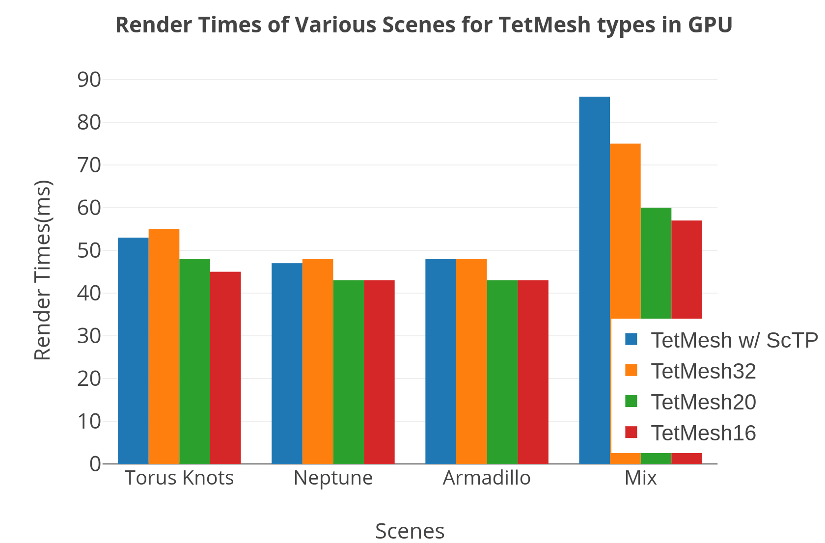
Figure 40: (Left) CPU render times; (Right) GPU render times for various TetMesh sizes over various scenes(increasing in complexity).
Weeks 18-20
This last homeworks topic was Path Tracing. The problem was fairly fundamental after writing a working recursive ray tracer. The big problem I faced was the mesh lights and the Light abstraction I previously had. Yet after fixing that everything worked out fine.
To begin with the problems I faced. My previous implementation of the light abstraction caused biased sampling for mesh light types thus resulting nasty artifacts(see Figure 41).
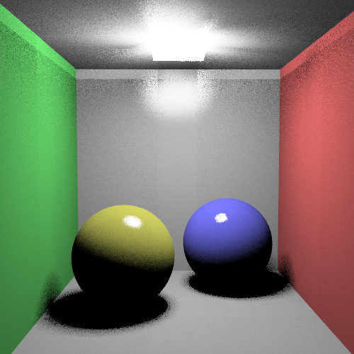
Figure 41: Lighting artifact due to biased sampling of mesh lights.
So what caused the problem?
Short answer:
I had a biased sampler for the mesh light source.
Long answer:
So basically my Light abstract class has two important functions:
SampleDirection(…) // samples a uniform random direction over the light source.
RadianceAt(…) // calculates the radiance at the given point using the light direction as a parameter from the first function.
My “genius” idea was to have the radiance calculated after the shadow tests thus gaining performance by not calling an O(1) function for every light source that needs to be sampled. Yet this started becoming problematic when I started working on area lights and mesh lights altogether.
The problem was when you try to sample a direction using the surface(just like the lecture videos) you can sample a point on the mesh where it is not visible to that point (a back face). And afterward, if you don’t keep that face for that ray you end up recalculating that face however accurately recalculating the sampled face is impossible. What I was doing was getting the closest face to the intersection point which MAY or MAY NOT be the face sampled in the SampleDirection(…) function. Thus causing bias in the selection, therefore, increasing the noise altogether.
After rewriting whole damn lighting abstraction to fit inside a singular function called SampleRadianceAt(vec3 isect_point, vec3 &l_vec). I was able to calculate radiance for the face picked along-side calculating a light direction that can be used as shadow ray direction. This fixed all of the noise issues even for the path tracer. Figure 42 illustrates the noise difference after I solved the issue.
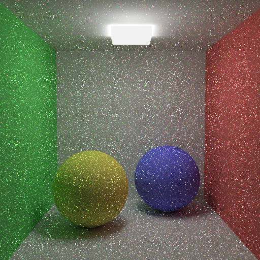

Figure 42: Noise in the path tracer due to biased sampling of the light source vs proper render with sample per pixel = 100.
Another minor problem I faced was mistakenly calling RecursiveTrace function in the PathTrace function as “recursion” I though I swapped all the function calls after I copied the method but I was wronng… As it turns out calls for dielectric/conductor materials were still RecursiveTrace calls.Whic caused inside of glass objects to be traced using direct lighting. One can observe this in Figure 43.
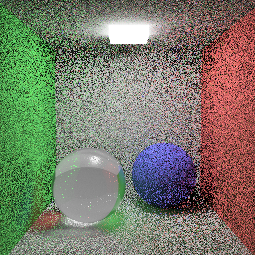
Figure 43: Inside of glass sphere is directly lit instead of path traced.
After swapping out function calls and implementing some simple techniques like:
- Russian roulette(RR) with throughput as the stopping condition,
- Importance sampling(IS),
- Next event estimation(NEE) for less noisy results
Final renders were ready. So here they are.
NOTE: There are 2 scenes for path tracing the combination of various techniques applied thus giving us 16 images. The order of these techniques in Figure 45 is:
- NEE
- NEE + RR
- IS + RR
- NEE + IS + RR
- none
- RR
- IS
- IS + RR
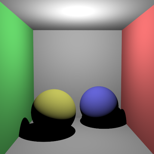
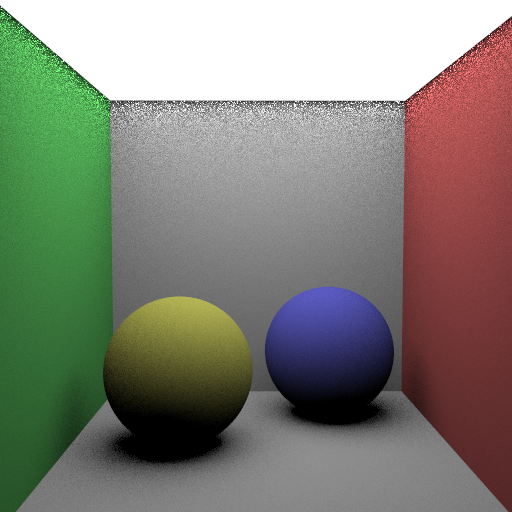
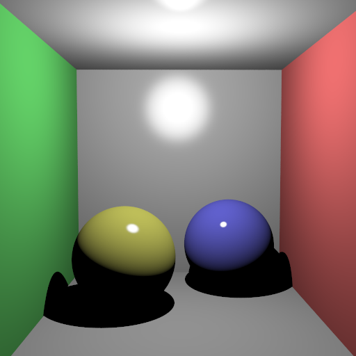
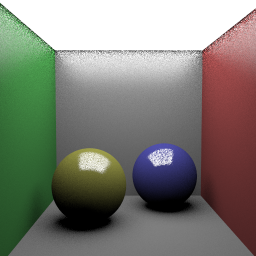
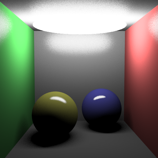
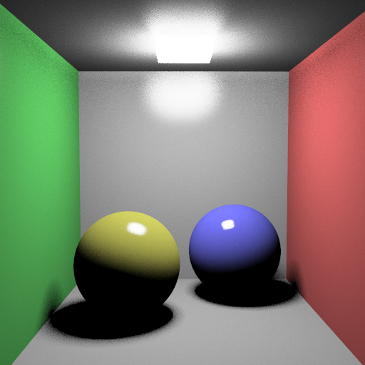
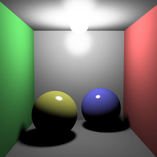
Figure 44: Cornellbox scenes with direct lighting raytracing
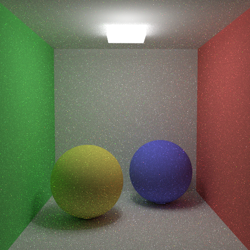
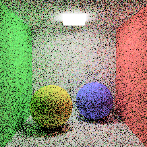
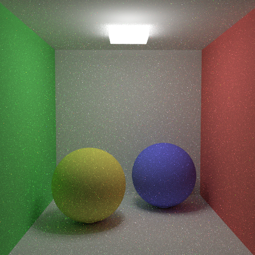
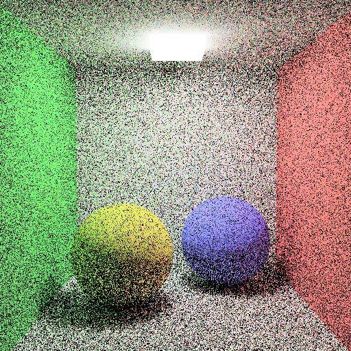
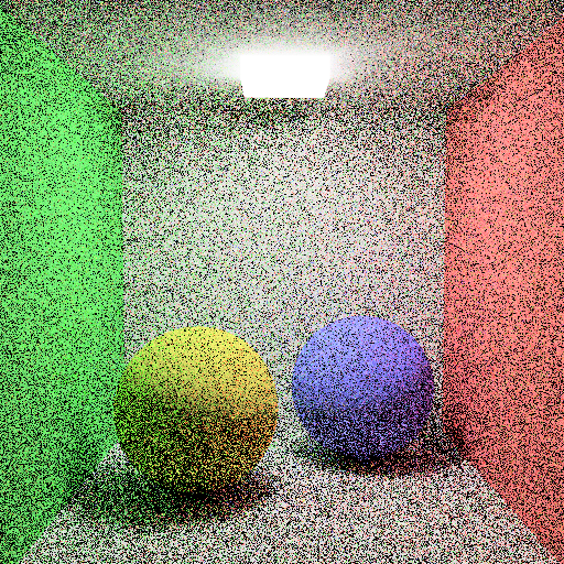
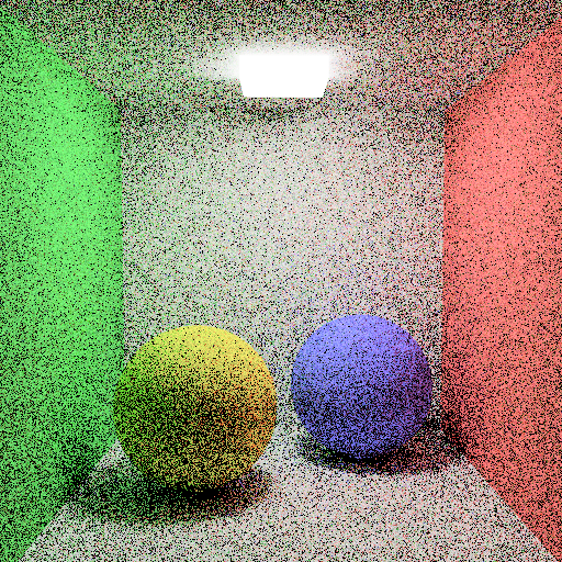
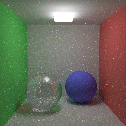

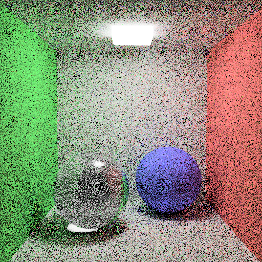
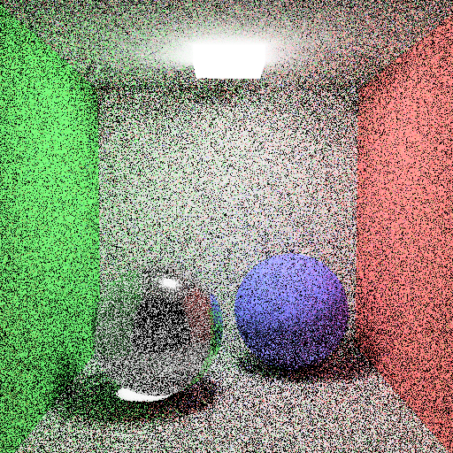
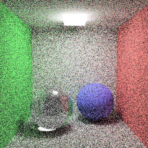
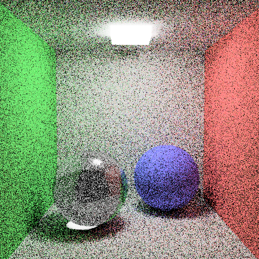
Figure 45: Cornellbox scenes with path tracing.
 Figure 46: Veach Ajar scene path traced with 1024 samples per pixel.
I also found some time to work on GUI tools that came in hand such as this little pop up that tells the information about the pixel the mouse is currently on.
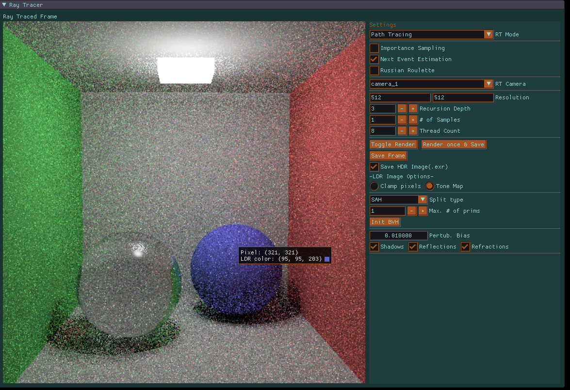
Figure 47: Pixel info gadget.
As for possibly the last entry to this blog I want to thank Associate Professor Ahmet Oğuz Akyüz(instructor for the CENG795 course) and Aytek Aman(PhD student at Bilkent Uni.) for teaching me so much about ray tracing and computer graphics in general.
References
[1]
Chroma-Works, “chroma-works/Chroma-Engine,” GitHub, 15-Aug-2019. [Online]. Available: https://github.com/chroma-works/Chroma-Engine. [Accessed: 07-Feb-2020].
[2]
T. Möller and B. Trumbore, “Fast, Minimum Storage Ray-Triangle Intersection,” Journal of Graphics Tools, vol. 2, no. 1, pp. 21–28, 1997.
[3]
Scratchapixel, Ray Tracing: Rendering a Triangle (Möller-Trumbore algorithm), 15-Aug-2014. [Online]. Available: https://www.scratchapixel.com/lessons/3d-basic-rendering/ray-tracing-rendering-a-triangle/moller-trumbore-ray-triangle-intersection. [Accessed: 18-Feb-2020].
[4] Scratchapixel, “Introduction to Acceleration Structures,” Scratchapixel, 08-Oct-2015. [Online]. Available: https://www.scratchapixel.com/lessons/advanced-rendering/introduction-acceleration-structure/introduction. [Accessed: 29-Feb-2020].
[5] M. Pharr, W. Jakob , and G. Humphreys , “Physically Based Rendering,” Physically Based Rendering, 2017.
[6] R. L. Cook, T. Porter, and L. Carpenter, “Distributed ray tracing,” Proceedings of the 11th annual conference on Computer graphics and interactive techniques - SIGGRAPH 84, 1984.
[7] K. Suffern, Ray Tracing from the Ground Up. Natick: Chapman and Hall/CRC, 2016.
[8] K. Perlin, “Improving noise,” Proceedings of the 29th annual conference on Computer graphics and interactive techniques - SIGGRAPH 02, 2002.
[9] E. Reinhard, M. Stark, P. Shirley, and J. Ferwerda, “Photographic tone reproduction for digital images,” Proceedings of the 29th annual conference on Computer graphics and interactive techniques - SIGGRAPH ‘02, 2002.
[10] AcademySoftwareFoundation, “AcademySoftwareFoundation/openexr,” GitHub, 27-May-2020. [Online]. Available: https://github.com/AcademySoftwareFoundation/openexr. [Accessed: 28-May-2020].
[11] Syoyo, “syoyo/tinyexr,” GitHub, 20-May-2020. [Online]. Available: https://github.com/syoyo/tinyexr. [Accessed: 28-May-2020].
[12] K. E. Torrance and E. M. Sparrow, “Theory for Off-Specular Reflection From Roughened Surfaces*,” Journal of the Optical Society of America, vol. 57, no. 9, p. 1105, 1967.
[13] A. Lagae and P. Dutre. “Accelerating ray tracing using constrained tetrahedralizations”. In 2008 IEEE Symposium on Interactive Ray Tracing, pages 184–184, Aug 2008.
[14]
A. Aman and U. Güdükbay. “Fast Tetrahedral Mesh Traversal for Ray Tracing”. In 2017 High-Performance Graphics Conference, July 2017.